How to Fix the #Spill Error in Excel (Step-by-Step)
#SPILL error occurs when there are not enough cells to populate the results of a function/formula.
If you’ve recently upgraded to Microsoft 365, you’d know that with a version upgrade, comes an error upgrade.
You’ll mostly see the #SPILL error in the dynamic Excel 365 as it produces dynamic arrays.
More details into what the #SPILL error is, what causes it and how can this be fixed in Excel come below 👇
So continue reading and download our free sample workbook here to tag along with the guide.
Table of Contents
What causes the #spill error
There are certain formulas whose results are not limited to a single cell. Their results extend across a range of cells.
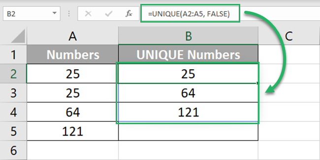
This range is called the spill range. 🌊 See for yourself:
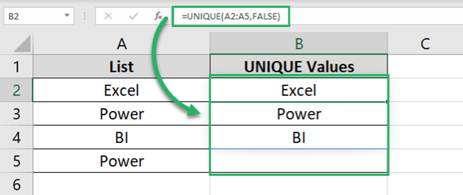
The UNIQUE function checks a list of items and returns the unique values of that list. This can be an array of values (just like B2:B4 in the image above).
Here Cell B2 to B4 make our spill range.
If this spill range is not vacant to populate the results of the UNIQUE function, we’d get the #SPILL error instead.

Pro Tip!
Check out the blue dotted border around the image above. When Excel returns the #SPILL error, it borders out the cell range needed to populate the results.
There’s not much guess game when it comes to the #SPILL error. It might only be caused by any of the following reasons 🤔
- The spill range isn’t blank. One or more of the cells in the spill range already contains some data.
- The spill range has some merged cells.
- The spill range falls in an Excel table. Dynamic arrays do not work in Excel tables.
- The spill range is too big. This is when the spill range goes beyond the boundaries of a spreadsheet.
- Excel fails to establish a spill range.
How to fix the #spill error
Fixing #SPILL errors in Excel is not that big of a problem. It simply depends upon what causes the error in the first place 🩺
To find the problem causing the #SPILL error:
- Click on the error icon next to the SPILL error.

- Check the option first in the consequent drop-down list.
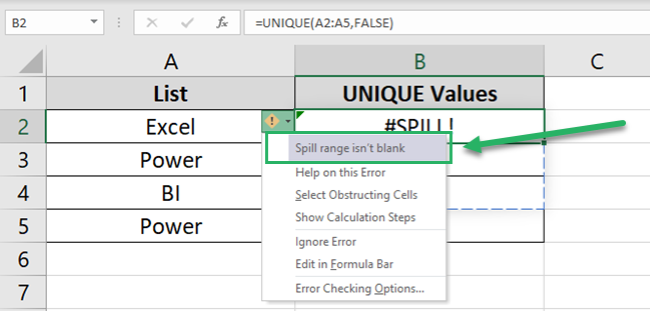
The problem here is the text “ABC” in Cell B3. And Excel has spotted the problem that the spill range isn’t blank.
Here are some solutions to fix the #SPILL error in Excel 🔧
The spill range isn’t blank
If the spill range isn’t blank, blank it out yourself.
As in the example above, the problem is caused by the text “ABC” in Cell B3.
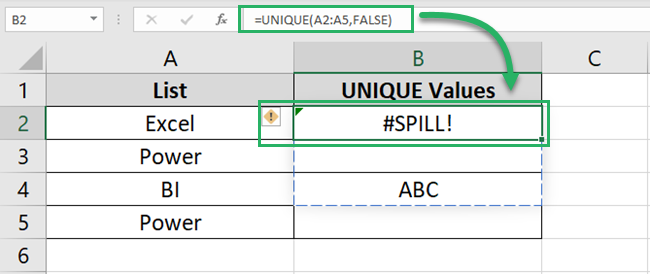
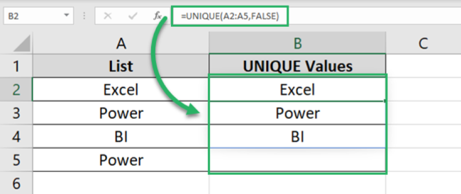
Delete it, and there you go!
The spill range has merged cells
Sometimes, you might get the #SPILL error because of merged cells in your spill range.
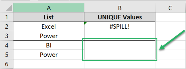
As in the image above, the problem is caused by the merging of Cell B3 and B4.
Unmerge them, and everything is fine 👍

The spill range is in an Excel table
Here we have an Excel table of numbers.
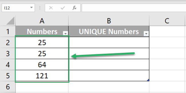
Note that the numbers and Unique numbers are in the form of an Excel table.
And we want to find the UNIQUE numbers from this list.
- Let’s then write the UNIQUE function as follows:
= UNIQUE (A2:A4, FALSE)
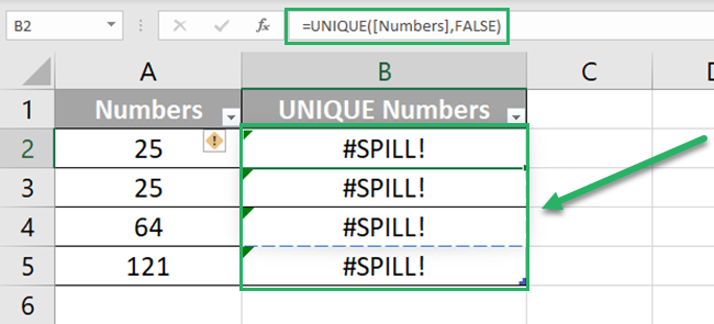
But we again have the #SPILL error 🥴
Note that this time the #SPILL error is not only in a single cell. But in all the cells of the range.
This is because the UNIQUE function is a dynamic array function. These functions are not supported by Excel tables ❌
So how to fix this? The only way you can help this is by converting your table into a normal range. To do that:
- Right-click anywhere on the table.
- From the context menu, go to Tables > Convert to Range.
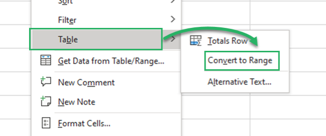
Once you have converted the Excel table into a normal range:
- Reapply the UNIQUE function, and it’s all sorted now.
Examples of formulas that return the #spill error
Most of the time, you’d see the #SPILL error for array functions. These functions result in an array of cells.
And if there are not enough empty neighboring cells to contain the results, you will end up with a #SPILL error in the formula cell.
You might turn a simple formula into an array formula too. Array formulas are those that give multiple results. These results may spill across the neighboring cells (down or to the right).
Here are a few examples of such functions and formulas:
Example No. 1: RANDARRAY function:
The RANDARRAY function is a dynamic array function.
It stands for a Random Array – and you guessed it right. It produces an array of random numbers🚴♀️
So, say we need an array of random numbers that is 5 rows tall and 4 columns wide.
Let’s write a RANDARRAY function in Cell A1 that gives us 5 rows tall and 4 columns wide array.
= RANDARRAY (5,4,0,100)
The first and second arguments are for the required number of rows and columns. The third and fourth arguments are for the minimum and maximum values that we need in our array.
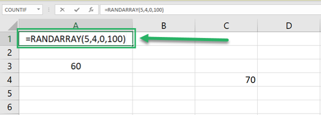
Note that the 4th row and the 3rd column in the image above already contain values 👀
And here are the results.
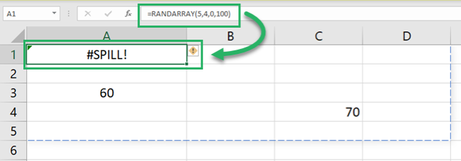
We only have a #SPILL error!
That’s because the resulting range had to spread across the 3 columns neighboring Cell A1 (Columns A to D). And 4 rows neighboring Cell A1 (that makes Rows 1 to 5).
But in our example, Row 4 and Column C already had data.
As all the required neighboring cells to populate the results were not empty – the RANDARRAY function returns the #SPILL error.
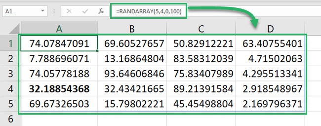
Now let’s clear out all the cells and write it again 🧹

This time the results are widespread.
Example No. 2: POWER Function
The POWER function is not a dynamic array function. It simply raises a number to a given power and returns the answer.
The same formula that we used in old-school math 👶
2 raised to the power 2 is 4.
Let’s do it here:
We have a list of numbers and we want to raise them all to power 2.
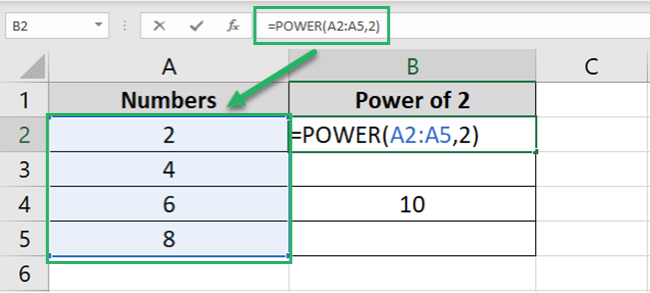
Let’s write the POWER function for all of them at once:
= POWER (A2:A5, 2)
The cell range A2:A5 contains all the numbers. Whereas “2” is the power to which these numbers must be raised.
Don’t forget to note that the list for powers is not empty. It already has a number in the third row.
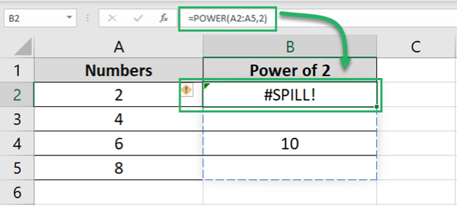
The POWER function fails to return the results as the spill range is not vacant 👆
Vacate Cell B4 and reapply the formula:
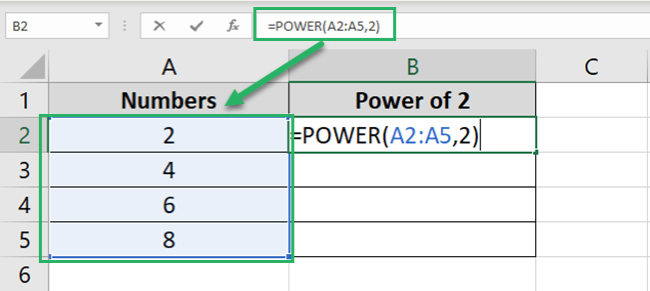
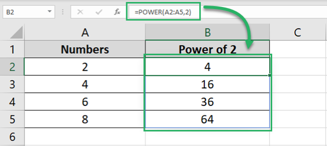
And this time, we get the POWER of all the numbers in one go.
Pro Tip!
Here’s something for you to note. Especially if you are an Excel user of older versions (more precisely, non-dynamic versions) of Excel.
If you apply the function = POWER (A2:A5, 2) in a non-dynamic version of Excel, you will not get an array of multiple values.
To get an array of results that automatically spills into neighboring cells in a non-dynamic Excel version:
- Write the formula
- And press Ctrl + Shift + Enter
Unless you press these three keys together, you’d only get the results for the first cell.
In dynamic Excel 365, this is no more necessary. You can simply press enter with the above formula and have your results ready 🎯
That’s it – Now what
The guide above mentions all the details about the #SPILL error. The causes, the fixes, some examples, and many tips 🤩
We have been on a rollercoaster ride of Excel learning, and let me tell you – there’s so much more coming.
Learning Excel is all about mastering Excel functions. And there are just so many of them. Some of my top favorite functions of Excel include the VLOOKUP, SUMIF, and IF functions.
Enroll in my 30-minute free email course today to learn these (and many more) Excel functions.
Other resources
There is a list of errors that you’d see in Excel when you work with functions and formulas.
To fix them, you must know what causes them in the first place. Read out our blog on the #VALUE, #NAME, and #Ref errors of Excel here.
