How to Show Formulas in Excel:
4 easy methods
Have you ever worked on a spreadsheet densely packed with formulas?
In such a case, to make sense of how each of the formulas works and how the results are derived, you might want to see the formulas in the cells.
This guide will teach you how to display formulas in Excel. 😀
Download our sample workbook here to follow the guide as we dive into the details of this topic.
Table of Contents
How to show formulas in Excel from ribbon
Type any formula into Excel, say = 2+ 2, and hit ‘Enter’.

It’ll take Excel less than a nano-second to run the formula above and display results.
But what if you want the formula ‘= 2 + 2’ to be on the display only? Here’s how you can do it.
1. Select any cell of your worksheet.
2. Go to the Ribbon > Formulas Tab > Formula Auditing group.

3. Click on the button ‘Show Formulas’.
4. Excel will now display the formulas for all cells in the worksheet and not the result.

Nice! How can we now get back the results?
5. Go back to the Ribbon > Formulas Tab > Formula Auditing group.
6. Again Click on the button ‘Show Formulas’, and there you go.

Excel again displays the result and not the formula.
Show formulas using the shortcut command
You can also display formulas in Excel by using a shortcut key. It is swift and easy.
1. Click any cell of an Excel worksheet.
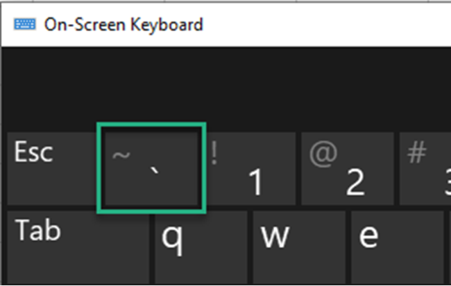
2. Press the Ctrl key + Grave Accent Key ( ` ).
Can’t find the grave accent key on your keyboard? Look to the left of 1 from the number keys.
This puts all cells of that worksheet to display formulas instead of the results.

Note that this shortcut only displays formulas for all cells of the active worksheet. Not the entire workbook.
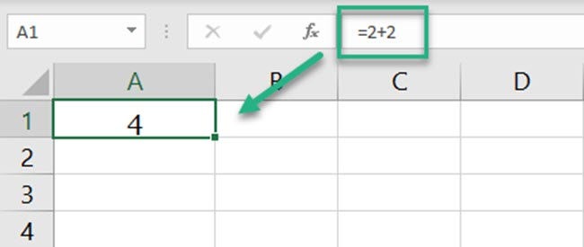
4. Want to go back already? Press the Ctrl key + Grave Accent Key ( ` ) again.
Excel takes the display back to the results. No more formulas.
That’s for Windows users. Does the method change for Mac users?
Certainly not. Even if you’re a Mac user, the process remains the same. Press the Control key + grave accent key (`) to display formulas.
Whenever you’re done and want to go back to the default display, again press the same keys together.
How to display formulas in specific cells only
We’ve come across two methods to display formulas in Excel already. However, did you notice something?
Both the above methods would display formulas for all the cells of the active worksheet.
But what if you only want to display the formula of a selected cell? There are two ways you can achieve this.
i. Add a space before the formula
Take the following image as an example, where cells A1, A2, and A3 have a formula.
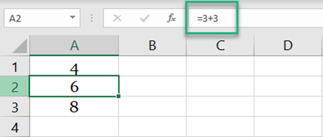
You want to display the formula for cells A1 and A2 only and not for cell A3.
1. Select Cell A1 and A2.
2. Go to Home Tab > Editing group > Find & Select > Replace.
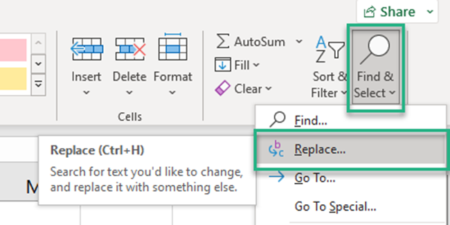
This launches the Find and Replace dialog box as below.
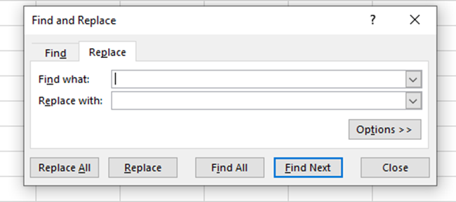
You may use the keyboard shortcut Control + H to launch the Find & Replace feature.
3. Against the Find tab, punch in an equal sign ‘=’.
4. Against the Replace tab, punch in an equal sign but after a space character ‘ =’.
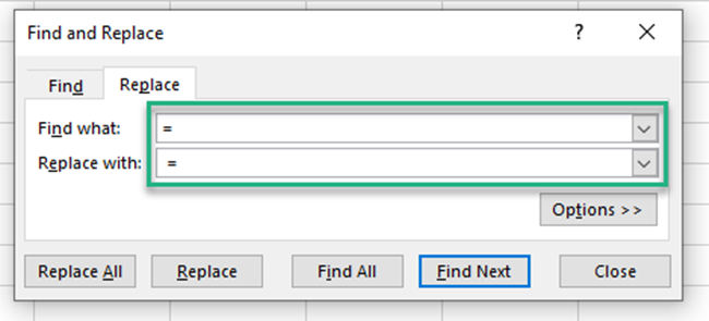
This way the formulas in the selected cells will not start with an equal sign but a space character. And Excel only recognizes a formula when it starts with an equal sign.
5. The results only in the selected cells will be replaced by formulas as follows.
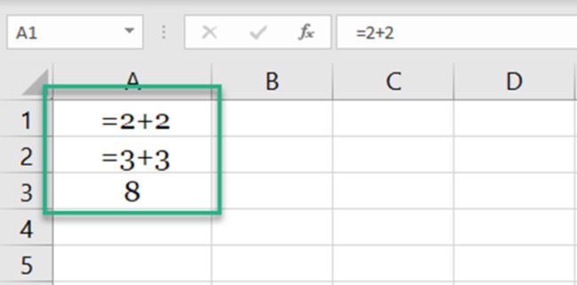
The selected range (Cell A1 and A2) shows formulas. Cell A3 continues to show the results.
ii. Add an apostrophe before the formula
If you do not want a space character visible in the cell, you may use this method instead.
1. Select Cell A1 and A2.
2. Go to Home Tab > Editing group > Find & Select > Replace.
3. In the Find and Replace dialog box, punch in an equal sign (=) against Find.
4. Against the Replace tab, punch in an equal sign but after an apostrophe (‘=).
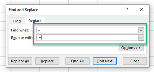
This way the formulas in the selected cells will not start with an equal sign but an apostrophe. Whenever something starts with an apostrophe in a cell, Excel takes it as a text string.
5. The results only in the selected cells will be replaced by formulas as follows.
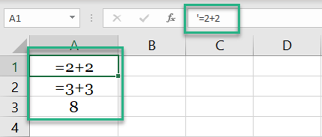
However, unlike the space character, the apostrophe is not visible in the cell. It is only visible in the formula bar or in the edit mode.
Pro Tip!
If you are in a hurry and only want to have a glimpse of the formula in a cell, the above methods might not suit you.
To check the formula to a cell, you may press ‘F2’. This will instantly show the formula running behind a cell.
However, as soon as you click away or press enter, the formula would be replaced by the result.
How to show formulas with the FORMULATEXT function
It’s time we introduce you to a modern-day Excel function. We bet you’ve not heard of it before.
The image below has a cell that contains a formula.
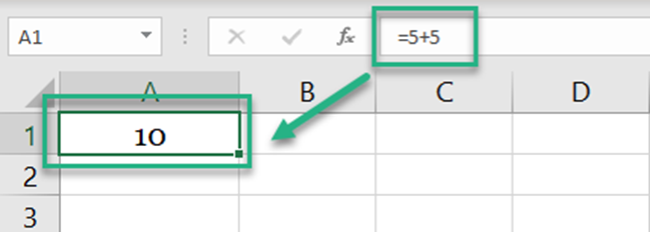
Do you want this formula to appear as it appears in the formula bar but in a different cell?
1. Activate a cell and write the FORMULATEXT function as follows.
= FORMULATEXT (A1)
Write that as the 2nd argument in the MATCH function, replacing what’s currently there.
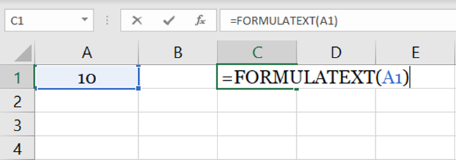
The FORMULATEXT function of Excel has a single argument – the reference argument.
In the reference argument, you create a reference to the cell whose formula you want to be displayed. We have created the reference to cell A1.
2. Hit enter to see the results as follows.
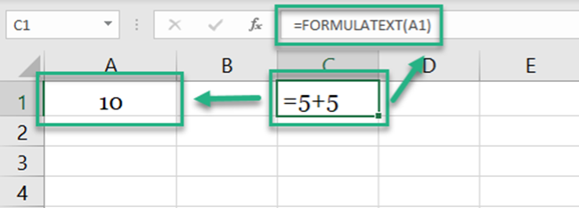
Note how Excel displays the formula of the referenced cell.
You can display the formula of any cell doing so. 😉
Pro Tip!
What if cell A1 above contained a formula with reference to another workbook?
The FORMULATEXT function would give back a #N/A error if that workbook is not open in the background.
How to select all formulas in the selection
If you’ve only received an Excel file prepared by someone else, how can you quickly identify the cells that have a formula running behind them?
The image below has a list of numbers (some of which are the result of a formula). Whereas, some others are simply punched in numeric values.
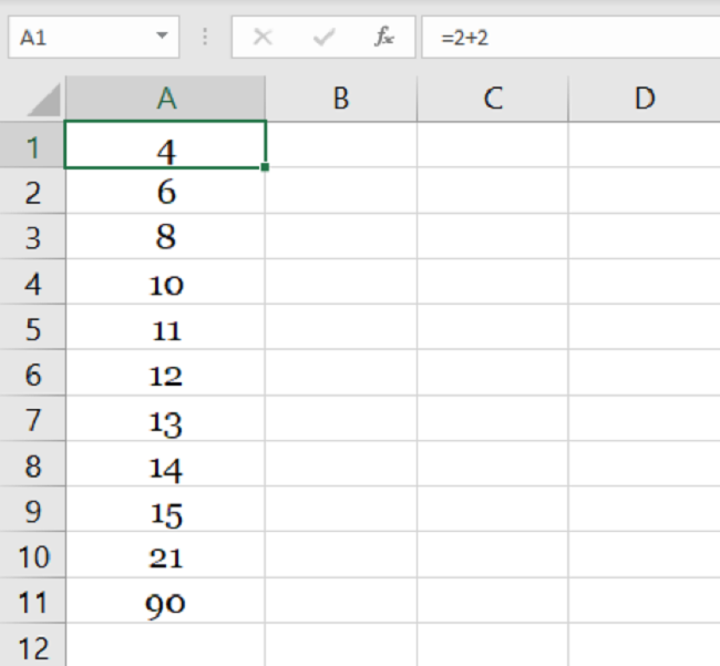
To select the formulas for the first six cells of this list (A1 to A6), follow these steps.
1. Select the cells (Cell A1 to A6).
2. Go to the Home Tab > Editing > Find & Select > Go to Special.
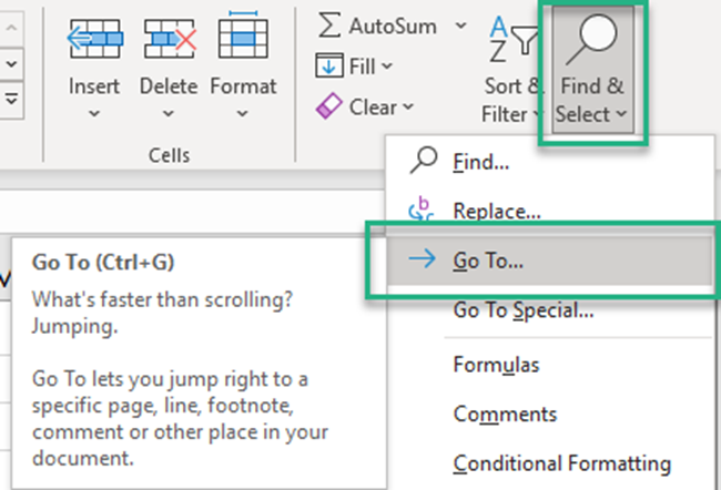
Or press down the Control key + G.
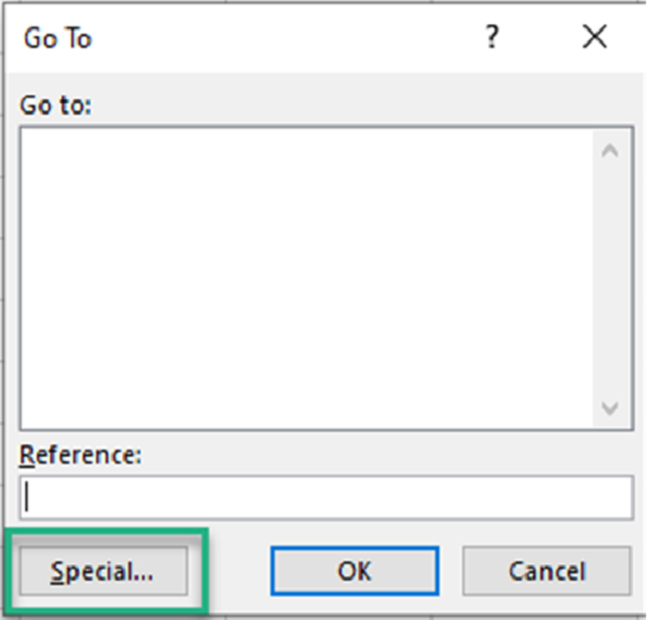
3. From the ‘Go To’ dialog box, click special.
4. Check ‘Formulas’ and press okay.
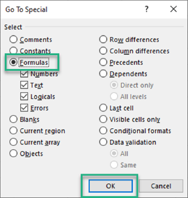
5. Excel selects all the cells that have a formula from Cell A1 to A6.
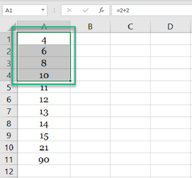
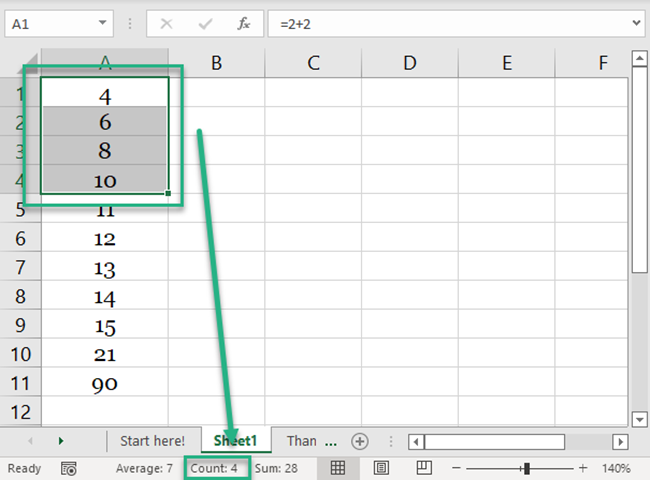
A5 and A6 do not have any formulas but only numbers. Hence, Excel did not select them.
You can format cells (highlight them) or check the count of these cells from the status bar.
How to print formulas
Whenever you print an Excel sheet, the print contains the calculated results. Not the formulas.
Need the print of your spreadsheet to have the formulas instead of the results?
1. Perform either of the methods above to display the formula in cells.
2. Once your worksheet begins displaying formulas, go to File Tab > Print..
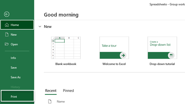
Or just use the print keyboard shortcut. Hit the Control key + P.
3. Here’s what the print preview looks like.

The final printed version would contain formulas and not their calculated results.
That’s it – Now what?
The tutorial above guides you on everything about formulas. Starting from displaying formulas in Excel to printing them.
Once you have a good grip on how formulas work in your spreadsheet, everything will begin to make better sense.
But, do you know how to use some of the most crucial formulas/functions of Excel? Like the VLOOKUP, SUMIF, and the IF functions?
Here’s my 30-minutes free email course that will help you master these and many more functions of Excel in no time.
Conclusion
Did this article help you gain better insight into Excel? If yes, we suggest you also take a quick look at some other relevant articles.
Like why formulas in Excel are not updating and how to keep formulas visible in cells. Keep coming back for more.
