How to Use Tables in Excel Step-By-Step With Examples
Not that you cannot get along in Excel without using tables – but if you yet don’t know what Excel tables are, you’re missing out on something very big 💥
Excel table is an amazing tool that will automate most of the operations that you’d want to perform on your dataset.
It is a named cell range that is a little too advanced when it comes to updating formulas, running totals, copying formulas, filtering, and sorting data.
The guide below will teach you all about Excel tables. So continue reading 🚀
And as you scroll down, do not forget to download our sample workbook here to tag along with the guide.
Table of Contents
What is an Excel table?
An Excel table is a named range that has a variety of features to manage and analyze data.
You can use it to run a calculated column, total rows, filtering, sorting, expansion, and whatnot. To help your curiosity, let us quickly show what an Excel table looks like 👀

Generally, a table is only a two-dimensional representation of data in the form of rows and columns 📝
Excel tables were introduced in Excel 2007 and are available in all next versions of Excel up to Excel 365.
How to create a table in Excel
Creating a table in Excel is the easiest of all. Let’s make one and see how this works.
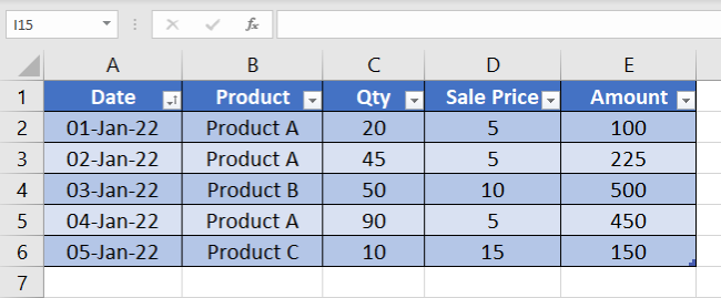
We have some data in the image below. Though it still looks like a table, note that this is not an Excel table yet.

To convert it into an Excel table 👇
- Click anywhere on the table.
- Go to the Insert Tab > Table.

If you’re more of a keyboard person, simply press down the Control Key + T to launch the create table dialog box ⌨
- The Create Table dialog box will automatically identify the cell range to be converted into a table.
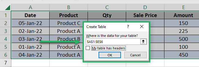
However, if that’s not your table exactly, you can manually adjust the range 🚴♀️
- Check the box for “My data has headers”. This refers to table headers.

- And Click Okay.
Your data is now converted into an Excel table and the default table style is applied 😍

Filtering Excel table data
Now that we’ve created a table out of our dataset, let’s see what we can do with it.
Our table has a list of sale transactions. Let’s filter out the sale transactions for Product A only 🅰
To do that:
- Click on the drop-down icon in the Products header.

- This will launch the Filter menu, as shown below.
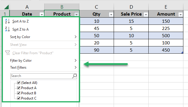
- Unselect all the products and only select Product A.
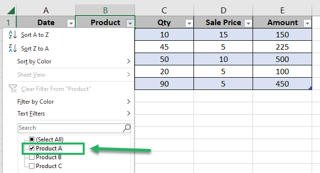
- And swish! We now only have the sales for Product A 🧙♀️

Similarly, you can filter the sales for any particular date or color by using the filtering option for tables.
Pro Tip!
The filter feature of Excel can be used without tables even. But for that, you need to manually select each column and apply filters to it 🥴
Excel tables bring you the advantage of an integrated Data Filter. However, if you don’t want your table to have them, that’s alright.
You can remove filters from your table in Excel by selecting the table > Table Design > Uncheck the Filter Button.
Sorting Excel table data
Excel tables also allow users to sort the data in their Excel tables in ascending or descending order 🔀
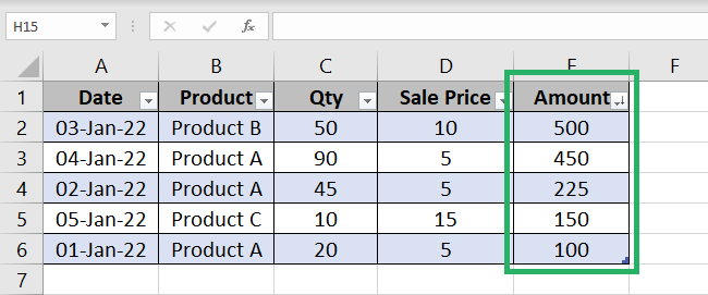
For example, let’s try sorting the sales in our table in descending order (largest to the smallest value). To do that:
- Click on the drop-down icon in the Amount header 📌

- From the drop-down menu, select the option “Sort Largest to Smallest”.
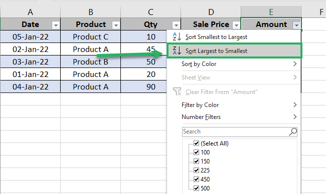
And look at the magic! The table looks all new instantly. The sale transactions are now organized in descending order in terms of the sale amount 🏆
You can do the same for dates – let’s sort them in ascending order.
- From the drop-down menu above, select “Oldest to Newest”.
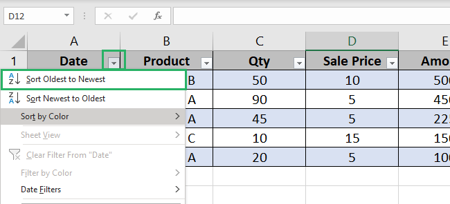
And see how the entire table is reorganized along with the dates 📅
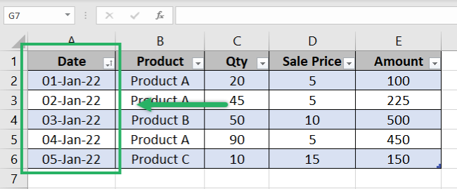
All the sale transactions are now arranged date-wise (from the oldest date to the newest one).
Format an Excel table
When you first create a table in Excel, it will appear in the default table format of Excel. Which you may or may not like 🙈
If it’s the latter case, don’t worry. You can reformat your table in a hundred ways. To change the format of your Excel table:
- Click anywhere on the table.
A new tab will appear on your Ribbon by the name of Table Design 🎨
- Go to the Table Design tab > Table Styles.

Those are not all.
- Click on the small arrow to the right of the table styles box to launch this menu further.
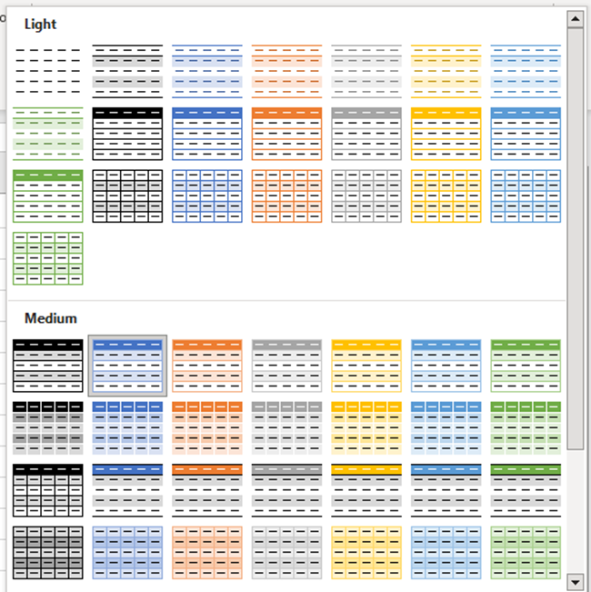
Too many. Aren’t they?
- Hover your cursor on these designs to get a quick preview of how your table will look under each design.
- Once you have chosen the design for your table, click on it to have it applied to your table.
Just like we have applied the light blue table style here 🥶
Summary row
Yeah, a summary row or you may call it the total row that you can add to your Excel table very easily 🔔
Let’s take the example of our table above, where we have the amount for sales in the last column. If you need to perform any operation on these sales – you don’t need to write functions from a scratch.
The Excel table will do that for you. See here.
- Select the table.
- Go to Table Design Tools > Check the option for Total Row.

- Check out your table for an additional row. Do you see the totals there in the right bottom?
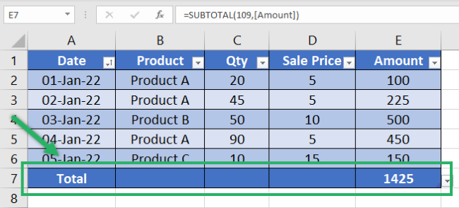
Not just the totals – but you can perform any function here 🤯
- Select the summary row for any column, and a drop-down arrow will appear.
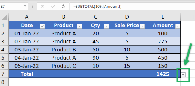
- Click on it to launch the menu of functions.
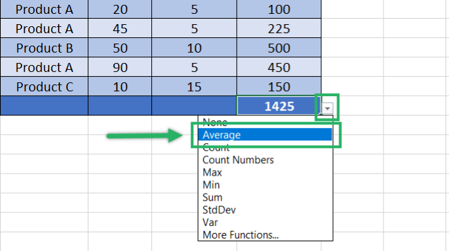
6. Choose any of these operations by clicking on it to have it applied to the subject column
For example, let’s try calculating the average sales by clicking on the Average option from the drop-down list.
And here comes the average for the above numbers 🔥
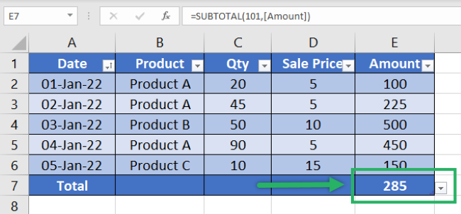
As easy as that.
Pro Tip!
If you go to the formula bar to see the function running on the backend of the summary row, you’d find the SUBTOTAL function instead of the simple AVERAGE function 🤔
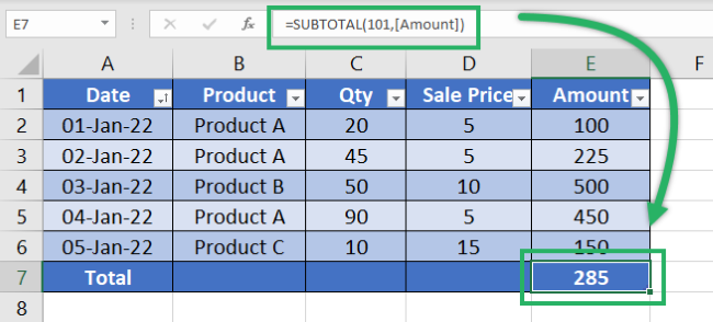
Why is it used, and why haven’t we used the simple SUM / AVERAGE functions?
Learn that by reading our blog on the SUBTOTAL function. Link in the Other Resources Section. 👇
That’s it – Now what?
Until now, we have learned almost everything about Excel tables. From converting a simple data range into a table to filtering, sorting, and formatting it.
Hope you enjoyed it just as much as we did. If you did, don’t just stop here 📍
Excel tables make a great tool that will ease your data storing and sorting jobs by 100 times. But that’s just one tool in Excel, and there’s a whole library of functions, features, and tools in Excel for you to explore.
To learn everything about Excel, master Excel functions first. Particularly, the key Excel functions like the VLOOKUP, SUMIF, and IF functions.
Other resources
If you learned reading about data tables in Excel, you’d love the Pivot Table tool of Excel too.
It is one of the most advanced tools of Excel that will take you by surprise. Read our blog on it here.
And here’s the link to the SUBTOTAL function discussed above. Dive right in by clicking here.
