How to Split an Excel Cell
(The Best Methods)
Often, when you import data into Excel from an external source, it reaches your sheet in a very clumsy shape 🤔
And sometimes, all the information comes merged within a single cell or column. If you’re going through such a situation, you’re not alone in this. Been there, done that.
To help such unorderly populated data, you’d need to split it into separate columns. This will make the data more readable, and help you sort it better.
But how to split cells in Microsoft Excel?
In this tutorial, I will show you how to do so by using the Text to Column feature of Excel alongside some other handy methods (the Flash Fill feature of Excel, and a combination of Excel Functions).
Grab your practice workbook for this tutorial here, and come along with me.
Split an Excel Cell using the Text to Column feature
The text to column feature of Excel is specifically designed to split cells in Excel.
It enables data segregation in Excel (from a single cell to multiple cells) within a split second that might otherwise take you hours.
I rate it as the best method to split cells in Excel as it allows splitting data in Excel into different cells based on delimiters such as commas, semicolons, space, and even fixed width.
Let me show you how it works through the example below.
Here we have some data populated in Excel that details on the new residents in a city 👨🦯
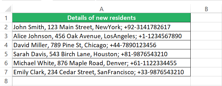
However, the problem with this information is that all their details are clustered together as a text string. This makes them almost impossible to process.
Here’s the format in which we need them populated ideally.
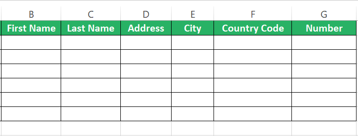
Ah-ah! Don’t start doing it manually already – let me show you how to make Excel do it using the Text to Column feature.
Splitting Cells with Delimiters
A closer look into the text string reveals that different information in the text string is separated through different delimiters.
To begin with, the name, address, and city related details for each new resident are separated through columns. To split them into different cells:
Step 1) Select the cell content to be split into multiple cells.
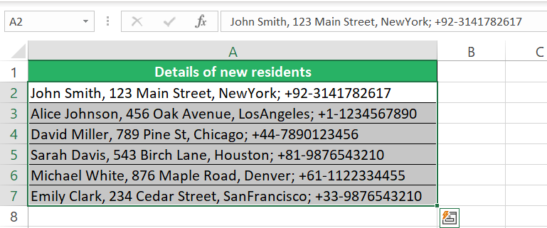
Step 2) Go to the Data tab > Data tools > Text to Column.

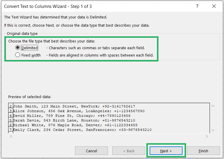
Clicking on it, you will get to see the Convert Text to Columns Wizard dialog box.
Step 3) Select Delimited and click the Next button.
Step 4) From the next window, select the Delimiter as “Comma”
You get a quick data preview at the bottom of how the split data would look like.
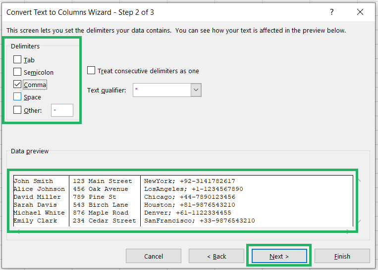
Step 5) Click on Next to see the following screen.
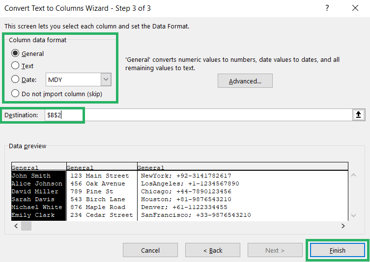
This is just about how you want the data in split cells to be formatted. We will keep the data format as General.
The General format automatically converts numbers to numeric values, date values to dates and keeps everything else formatted as text. Hence, it’s safe to go with the General dat format as of now.
Step 6) Choose the destination cell as $B$2 (from here onwards the data will be placed).
It is important to define the destination cell, or else Excel might overwrite the original existing data (like the original data in Column A).
Step 7) Click Finish to have the following results.
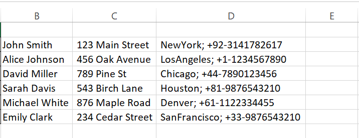
Cool! So, we have the full names, addresses, and [city + country code + cell number] separated 💪
Next, we need the first and last names split into different cells. For that:
Step 8) Add a column after the column where names are populated (Column B).
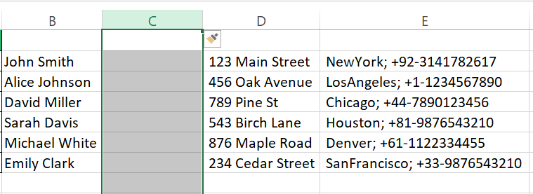
Doing so will keep the data in harmony and the last names would appear in Column C.
Step 9) Select the column containing the names and go to the Data tab > Data Tools > Text to Column feature.
Step 10) Again select “Delimited” and go to the Next button.
Step 11) From the Delimiters, select “Space”. This is because the first and the last names within each text string are separated by a space character.
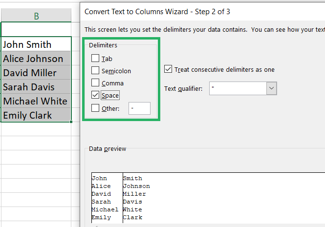
Step 12) Click on the next button, and select the data format as “General”.
Step 13) Select the destination cell as $B$2 (the new column we added) and click on “Finish”
And there we have it, first and last names split into different cells.
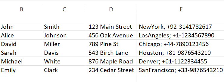
We are very close to having our data sorted. Just one more round to go! 🏍
We now need to separate the city, the country code, and the phone number.
Since the city and the phone number are separated through a semi-colon (;), repeat the steps above until you reach the delimiter window as below.
Step 14) From the Delimiters, select “semi-colon”.
We also need to split the country code (+1, +92, etc.) and the remaining phone numbers that are separated by a hyphen (-), so:
Step 15) From the Delimiters, also select “Other” and in the box next to it, type in a hyphen (-).
Excel offers some delimiters like commas, spaces, tabs, and semi-colons built within the Text to Column feature. However, if your data has other separators (like the hyphen above), you can input that manually into Others.
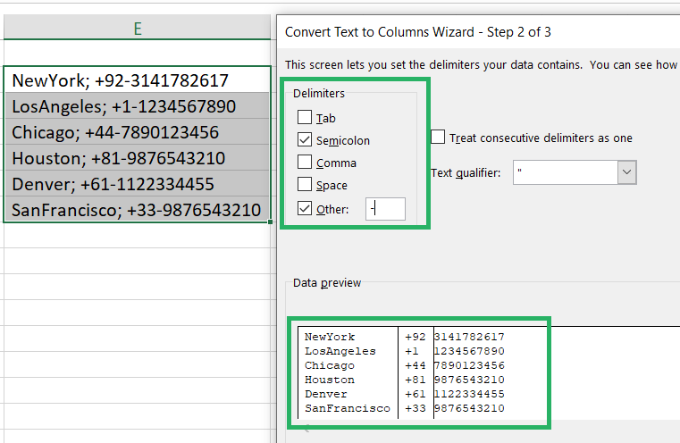
Step 16) Define the data format and the destination cell as $E$2.
Step 17) Click on “Finish”
There it goes.
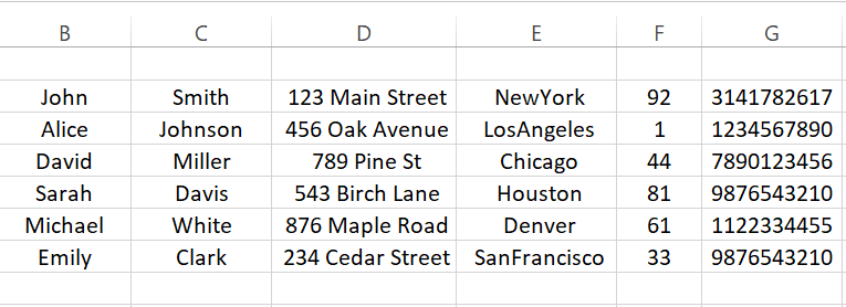
Very nice – except for a problem. Since Excel treats these values as numbers, it takes a plus sign preceding the country code as a positive value and eliminates it upon splitting 👀
No worries. We will fix it just now.
Step 18) Select the column for country codes.
Step 19) Go to the Home tab > Number > More Number formats > Custom.
Step 20) Set up the following Custom format for it.
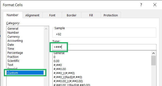
This custom format tells Excel to add a plus (+) sign before the number in each cell.
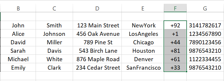
Adding headers and some formatting. And the data looks all clean and sorted – just like we wanted it.
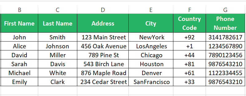
Delimiters make cell splitting in Excel real fun – don’t they? Plus, they save on tons of time and effort.
Splitting Cells using Fixed Width
Another way how you can use the Text to Column feature of Excel is by splitting your data based on its width.
If you have data in Excel that look alike in width like below:
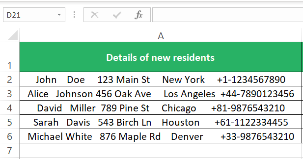
You can launch the Text to Column window and:
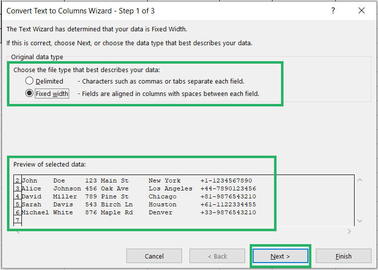
Step 1) Select Fixed Width and click on Next.
Step 2) In the Preview Pane, add and move the scale to define the points where Excel should split data.
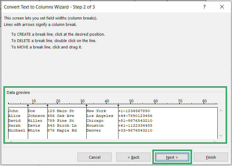
Step 3) Go to next and then the Finish button.
Here’s how Excel splits data into different cells based on a fixed width.
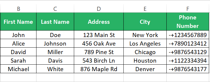
Splitting cells based on their Fixed Width can only be of use for cells with homonymous data. If the data to be split doesn’t run a similar width, this feature might not work very well for you.
Other Methods to Split Cells in Excel
That’s not it – there are other methods too that you can use to split cells in Excel 📝
Flash Fill
Flash Fill is one of the smartest features of Excel and I love using it.
To split cells in Excel for the same dataset as above using the Flash Fill feature:
Step 1) Add a new column next to the column where the data is populated.
Step 2) Begin writing the first name in the new column for the first few cells.
Step 3) As soon as Excel recognizes the pattern, it will populate the remaining cells for you. Like here.
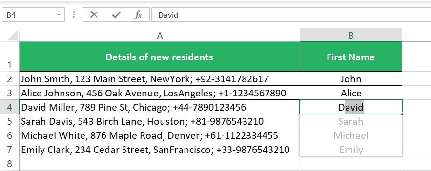
Step 4) If the results populated by Excel are those that you desire, just hit Enter and Excel will do the rest for you.
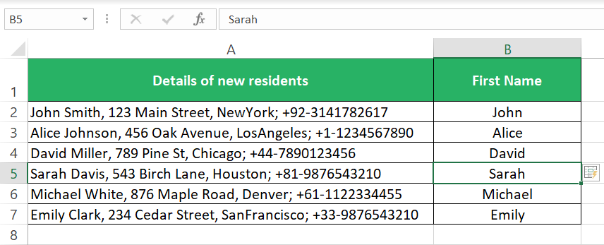
This we call the Flash Fill feature of Excel – it senses a pattern of how you’re filling in cells and does it for you in a blink.
Substring Extraction using formulas
You can also split cells in Excel by using a combination of Excel formulas / functions.
For example, in the above example, to split the first name into a different cell, we need to extract text substrings from the left of the cell.
So, we will use the LEFT function as follows 📌
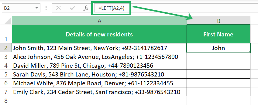
Similarly, you can use the RIGHT and the MID function to extract substrings from the mid and right of a cell value.
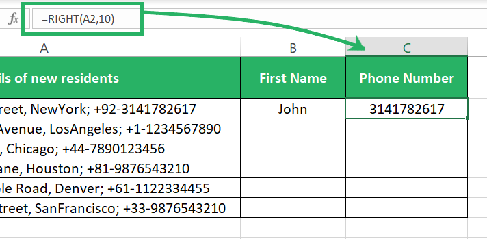
Taking it a step forward and combining it with the FIND and LEN functions, you can almost automate the substring extraction in Excel.
Read my blog here on Substring Extraction in Excel using TEXT functions to learn everything about it.
Conclusion
If you’re someone who gets to deal with data, splitting an Excel cell into multiple cells is something you’d often have to encounter 🏸
The different methods to do so in Excel discussed above will prove super useful for you in such circumstances. But why only these, there’s so much more about data cleaning and processing in Excel that you must learn.
My following blogs from data processing in Excel are undoubtedly my favorite.
- How to Use Data Validation in Excel: Full Tutorial (2024)
- How to Sort Columns in Excel (Without Mixing Data)
- How to Transpose Data in Excel: Turn Rows into Columns (2024)
Do give them a read. Hope you enjoyed the above tutorial and found all the information you’ve been looking for.
