How to Use Wildcards in Excel: Examples with VLOOKUP, COUNTIF, + more

Wildcards are some special characters that play the role of joker cards in Excel🃏

How? You can use them as a substitute for any character you are unsure about. By doing so, you can do so much in Microsoft Excel which would have been impossible (or at least very difficult) otherwise.

To learn all about using wildcard characters in Excel, continue reading the guide below.

And as you move forward, download our free sample Excel workbook here to practice side by side.

How to use wildcards in Excel

There are a total of three wildcard characters in Excel.

• asterisk (*)
• question mark (?)
• tilde (~)

Each of these characters has a different use. You can use them to perform partial matches. Or as a comparison criterion to filter data or to find common values.

Let’s see how you can use each of these wildcard characters through the examples below.

The asterisk wildcard character

The first and the most dynamic of all, an asterisk is used as a substitute for any number of characters.

For example, if we use an asterisk with a word as (Ma*), it will represent all the strings that start with the two alphabets “Ma”. These could be Man, Matter, Match, and any word that starts with the alphabets “Ma”.

Time we see it working in Excel? Check the image below that has a list of fruits.

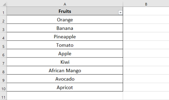
The data above contains a few fruit names that end with the letter ‘e’. Can we readily filter these out? Here’s how you can do it:

1. Select the column header of your dataset.
2. Go to Data > Sort & Filter > Filters.
3. Once you have the filters applied, click on the drop-down menu icon to launch the filter menu.
4. In the search bar, write the filter criteria as follows:

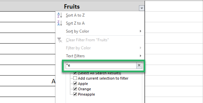
An asterisk with an “e” tells the Excel filter to show every value with an “e” at the end. Irrespective of the number of characters that come before “e”.

And here comes the magic of the asterisk. ✨

Excel filters out all the fruits that end in the letter “e”.

Pro Tip!

What you must notice is that each fruit has a different spelling.

• The word “Orange” has five letters to its name before the letter “e”.
• The word “Pineapple” has eight letters to its name before the letter “e”.
• The word “Apple” has four letters to its name before the letter “e”.

But regardless of the number of characters before “e”, Excel filters all the words ending in “e”.

Pretty cool, right? 🤩 This was just one example of its use. An asterisk can be used in place of any character, in any position.

For example, from the same list of fruits, what if you want to filter out fruits beginning with the letter “A”?

To do so:

1. Launch the Filter Menu.
2. Define the filter criteria as:

a*

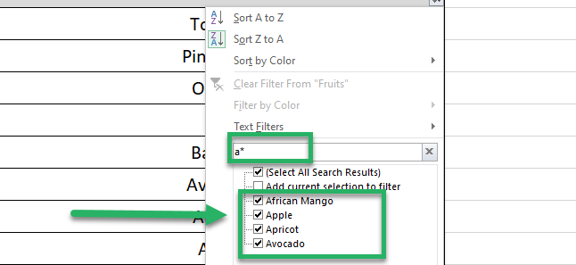
Here, we need to filter out fruits starting with the letter “A”, irrespective of the number of characters in the name of the fruit after A.

So the criteria is an asterisk after A (a*).

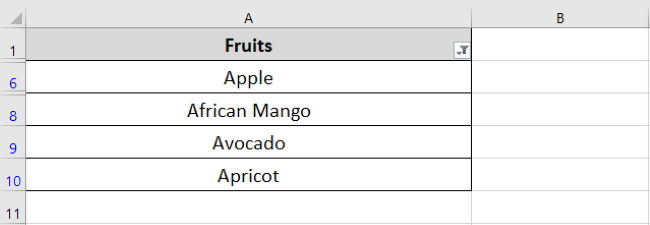
3. Hit Enter and there you go.

All the words starting with the letter “a” are filtered out.

Pro Tip!

Wildcards can be used even when you are unsure about the letter case.

Like in the above example, we defined the criteria as (a*). Whereas, the fruits in the list above start with a capital A. The results, however, remain unchanged.

The question mark wildcard character

A question mark is used to substitute a single unknown character.

For example, here is a list of words (some of which start with the alphabet S and end in N).

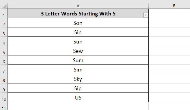
From this list, can we filter out all the three-letter words that start with “s” and end with “n”?

To do so, we must replace the middle character of “S” and “N” with a question mark as shown below.

s?n

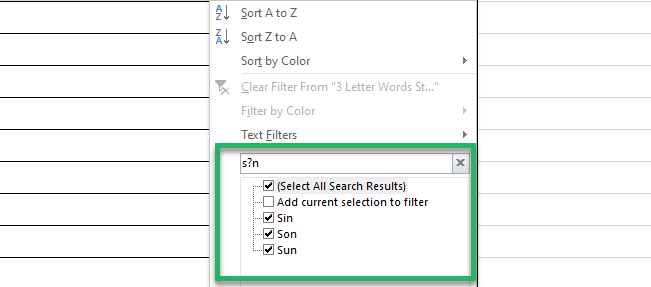
This tells Excel to filter out all the words that start with “S” and end with an “N” with any single character in between.

And here come the results.

Interesting, isn’t it?

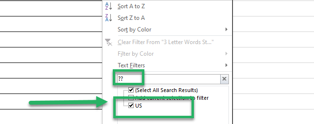
And what if we want to filter out words that have two characters?

Simple – Type “??” in the filter box and Excel will filter out all two-letter words as shown below.

The tilde wildcard character

Until now, we have seen how helpful the above two wildcard characters are. But what if you want to use them as literal characters and not as wildcard characters?

This is where the tilde comes in. It allows us to use the asterisk as a literal asterisk or a question mark as a literal question mark.

See the tilde work in Excel below.

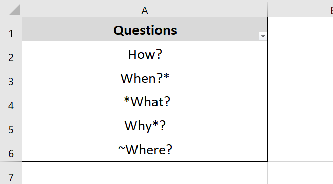
The data in the image above has words with asterisks, question marks, and tildes in them.

Let’s see what happens when we type a question mark in the filter box.

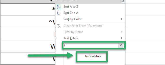
No matches? Huh.

Excel considered the question mark as a wildcard character. Doing so, it only looks for single-character words – and the data has none of them so you pull off nothing.

But what if we want Excel to filter the values ending with a literal question mark?

Let’s try using a tilde ‘~’ before the question mark.

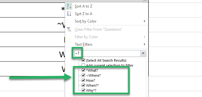
In this search, the filter results contain all the words with a literal question mark.

In the filter criteria box, add another tilde to the tilde as shown below.

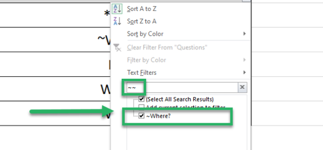
And you see the results. Excel finds the words containing a tilde.

So technically a tilde nullifies the effect of other wildcard characters. Funny, isn’t it? 😁

Using wildcards with Excel formulas

Till now, we have learned the general use of Excel wildcard characters.

But that’s not it. Wildcard characters are the most useful when used in pair with other functions of Excel.

Most importantly, the VLOOKUP, and COUNTIF functions. Time we see how to do so? Let’s dive into it.

How to use wildcards with VLOOKUP

Using the VLOOKUP function, you can search for a value from any dataset in Excel.

That’s true – but how can you use the VLOOKUP function when you are unsure about the value to be looked up?

Using the wildcard characters 🎯

The data in the image below has a list of locations – and for each of them, we want to find the number of umbrellas sold.

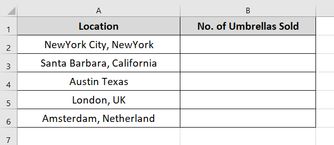
The number of umbrellas sold sits in another dataset (the lookup table) as shown below.

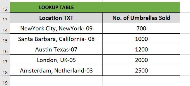
We want to match our entries in the ‘Location’ column with the ‘Location TXT’ column in the lookup table.

But here’s a problem – the lookup table has certain codes at the end of each location’s name.

Applying the VLOOKUP function using the names of locations only won’t yield us a thing. See for yourself.

We have set up the VLOOKUP formula that tells Excel to return the number of umbrellas sold in NewYork City from the lookup table.

= VLOOKUP (A2, A13:B18, 2, 0)

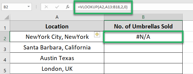
And guess what? Excel only returns the #N/A error. This is because the lookup table doesn’t contain simple locations but locations with codes.

To help this situation out, we need to perform a partial match. So, rewrite the VLOOKUP function as follows.

=VLOOKUP(A2&”*”, A13:B18, 2, 0)

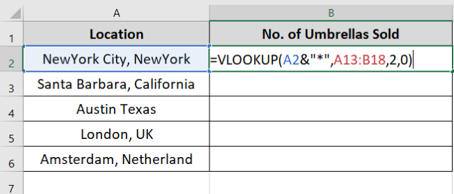
Did you notice something different about the above function? The lookup value.

We added an ampersand (the concatenate function) next to our lookup value, followed by an asterisk.

So technically, we changed the lookup value from simple A2 (location name) to A2&* (location name and any number of characters after it).

Excel now looks for all values that have NewYork City, New York to them. Irrespective of what comes after this text string.

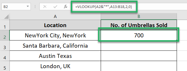
And Ta Da! Excel finds the number of umbrellas sold for NewYork City from the lookup table.

Turn the lookup table reference into an absolute reference. And drag and drop the results to all the locations.

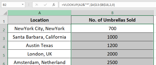
Excel finds and returns the number of umbrellas sold for each location.

Even though we didn’t know the exact codes for each location, the asterisk replaced it and helped us extract the results based on a partial match. ✌

Pro Tip!

Do you know about the XLOOKUP function? It is the advanced version of the Excel VLOOKUP function.

The XLOOKUP function offers an in-built mode for performing wildcard character matches. And so, you don’t have to embed wildcard characters into the search criterion to perform a partial match as above. 💯

How to use wildcards with COUNTIF

Using wildcards with the COUNTIF function brings you a whole new level of ease.

Let’s see how through the example below.

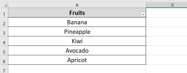
Here comes a list of fruits. And this time, we want to count the fruits with seven characters in their name.

To do so, write the COUNTIF function as follows:

=COUNTIF(A2:A6,”???????”)

The above function tells Excel to find strings with any seven characters from the range A2:A6.

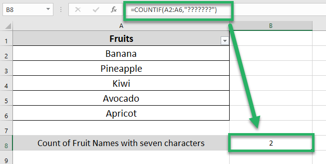
Excel returns the count of 2. The above list has two fruits with seven characters to their name.

Which ones by the way? (Avocado🥑 and Apricot 🍊).

And what if we change the formula to,

=COUNTIF(A2:A7,”?*”)

This tells Excel to count the number of fruits (words) that have:

• a single character (at least) and;
• any number of characters (at most).

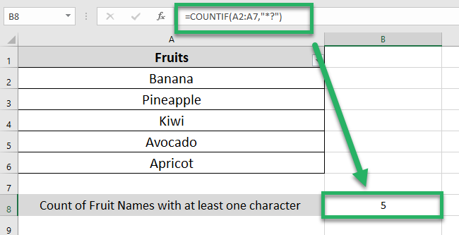
Excel counts all the fruits as they all meet the criteria defined above.

Note that in the range of cells to be counted, we have also included a blank cell (cell A7). However, this cell is not counted by Excel as it doesn’t meet the defined criteria.

That’s it – Now what?

The guide above runs us through the smart use of Excel wildcard characters through practical examples. We also learned to use them together with two important Excel functions.

But that’s not it – there are several more ways how you can use wildcard characters in Excel. For example, with the find and replace feature of Excel. 💪

Some other functions of Excel where wildcard characters can come in handy include the SUMIF, IF, and VLOOKUP functions (advanced uses).

Need help figuring out where to start learning these functions? You’re just one click away from it.  Click here to register for my free 30-minute email course to learn these and many more functions of Excel.

Other relevant resources

Need to learn more about the amazing uses of wildcard characters?

Hop on here to learn to use wildcard characters in the find and replace feature of Excel. You can also use wildcard characters to extract the first word in Excel.