How to Add Yes or No Options in Excel (Drop-down & Box)
When you’re setting up a workbook to share with others or for other collaborative purposes, you often want to control the information others can input.
It could be a defined range of data, certain numbers or text strings, and sometimes, just a simple “Yes” or “No” 🤚
This saves data entry time for users and guides them on how to populate the spreadsheet. You can restrict the input in your sheet to specific values by creating and implementing data validation rules.
In this tutorial, we will see how to add “Yes” or “No” Options in MS Excel as a drop-down list. To learn it along the way, download the free practice workbook for this guide and read it till the end.
Add Yes or No Options in Excel by entering them manually
The first method how you can create drop-down lists in Excel is by adding the options to it manually.
And it is super easy 😃
Here I have some questions from a survey form in Column A, where the answer can only be a Yes or No.
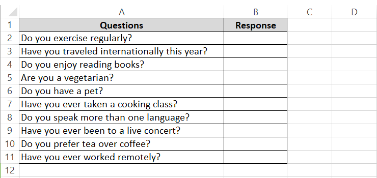
To create a drop-down list of the answering options for these questions, we will follow these steps:
Step 1) Select the first cell where you want the drop-down box inserted.
Step 2) Go to the Data tab > Data Tools group > Data Validation.

It will open the Data Validation dialog box 📝
Step 3) In the Data Validation box, go to the Settings tab and define the Validation Criteria as:
- Allow: Select List
- Check the Ignore Blank and In-cell dropdown checkboxes
- In the Source field, write Yes and No separated by a comma.
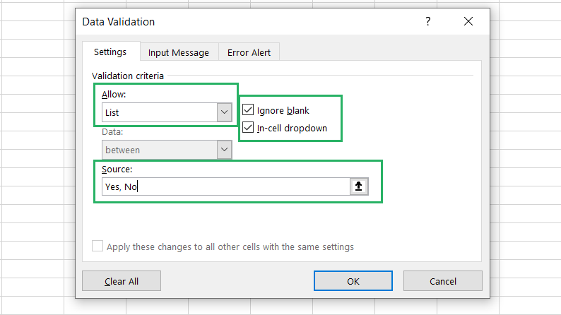
Step 4) Click Okay.
A drop-down menu will be added to the selected cells with the pre-defined list of options (i.e., Yes and No). Users need to click on the small drop-down arrow on the cell’s right to launch it.
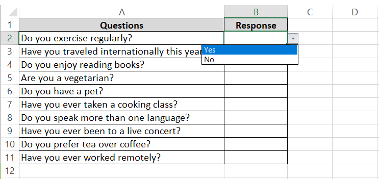
Wow! Looks so cool ✌
Step 5) Now to add this drop-down list to the remaining cells, drag it down to all the cells.
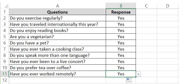
This is one quick way to add your drop-down list to several adjacent cells. However, this can also be done to non-adjacent cells by copying and pasting the cell that contains the drop-down list. We will cover that method in a later section.
Let me show you how the drop-down list works.
If I select any options from Yes or No or type either of these in this cell, it will be added to the cell.
But if I attempt to write anything other than these pre-defined options, Excel will return an error message like this 🚫
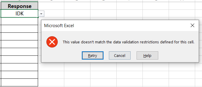
This way you can restrict the input of values other than those defined by you.
Also, if you do not want a harsh error message like the above but something more subtle (or anything else), you can get it by customizing the error message below.
Step 1) Select the cell (or cells) where the drop-down box is inserted.
Step 2) Go to the Data tab > Data Tools > Data Validation.
It will launch the Data Validation dialog box.
Step 3) In the Data Validation box, go to the Error Alert tab.
Step 4) Select the style as anything from Stop, Warning, or Information.
Step 5) Define the title and Error message as you like.
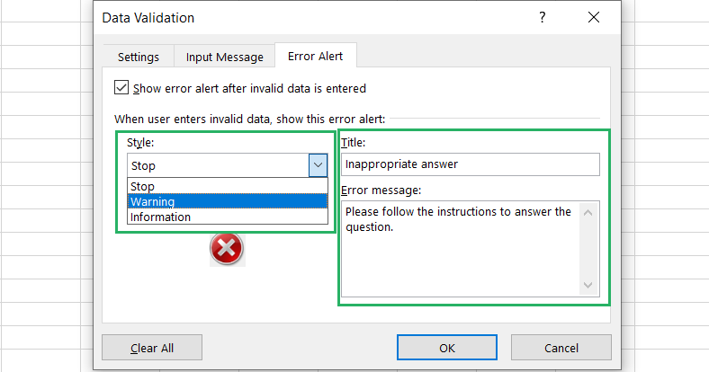
Step 6) Click Okay.
Now the next time any user tries to write any option other than the pre-defined ones in this cell, Excel will return the defined error message ✍
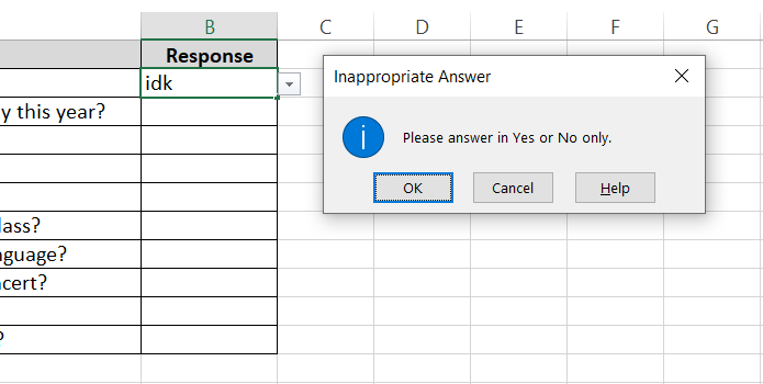
Similarly, you can define an input message to appear next to this cell to guide users on how to populate these cells.
Step 1) Go to the Data tab > Data Tools > Data Validation.
Step 2) In the Data Validation box, go to the Input Message tab.
Step 3) Define the title and Input message as you like.
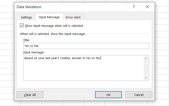
Step 4) Click Okay.
Every time a user hovers his cursor around this cell to select an option, this Input message will appear in a small yellow flap towards the right.
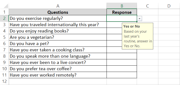
Makes this whole process so much fun as you can customize every aspect of drop-down boxes to your choice.
Add Yes or No Options in Excel by referring to a cell range
Although we are dealing with a simple Yes or No case at the moment, sometimes you might have a range of options and manually typing them in the Data Validation box might not be the best option 🎯
For such a case, you can define these options in a cell range and then refer to it as the source of the drop-down box.
See here:
Step 1) Enter data (Yes and No) in any cells of your sheet.
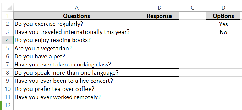
Step 2) Select the cells where you want the drop-down box inserted.
Step 3) Go to the Data tab > Data Tools > Data Validation.
It will launch the Data Validation dialog box.
Step 4) In the Data Validation box, define the Validation Criteria as:
- Allow: List
- Check the Ignore Blank and In-cell dropdown checkboxes
- In the Source box, refer to the range of cells where you have input the options or select them and Excel will automatically get their reference (D2 and D3)
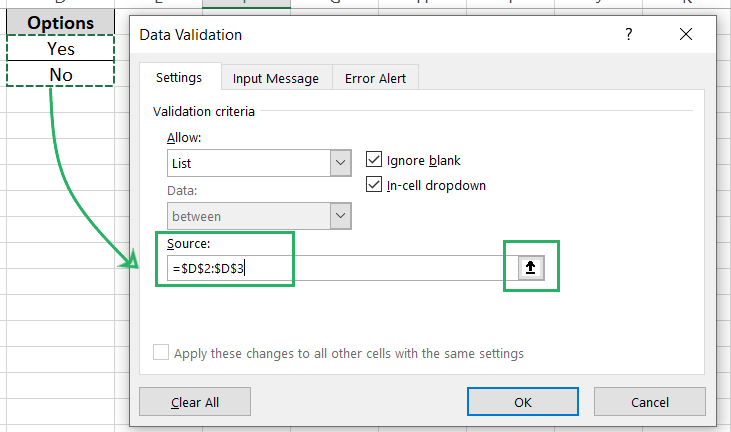
Step 5) Click Okay.
You’d see a drop-down list pop-up with these options will be added to the selected cells.
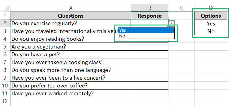
This is a preferable option for when you have a long list of options to pre-define.
Copy and Paste Yes or No Options to other cells in Excel
The best part about drop-down lists is that you can copy and paste them into multiple cells.
I showed you how you can expand your drop-down list in Excel by dragging it down the list in the first section. This method will work (and might be better) for adjacent rows and columns 🤿
But if you want to add these lists to non-adjacent cells, it will not work.
For such cells, you can copy and paste a cell that contains this drop-down list.
Step 1) Copy the cell by pressing the Ctrl key + C key.
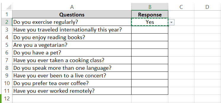
Step 2) Select the cells where you want it pasted.
Step 3) Press the Ctrl key + V key to paste it into those cells.
You will see the drop-down list copied and pasted to all the selected cells.
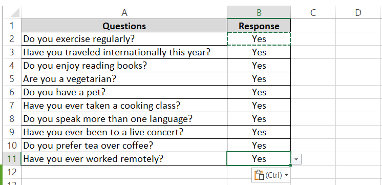
This was a simple case where you just copied a cell and pasted it down the list.
But such simple copying/pasting copies and pastes all the contents of the copied cells (including the formatting).
In the case above, the destination cells didn’t have any specific formatting, so this was not a problem 👀
But if you want to preserve the formatting of the cells where the drop-down list is being pasted while you paste the drop-down list, follow these steps:
Step 1) Copy the cell by pressing the Ctrl key + C key.
Step 2) Select the cells where you want it pasted.
Step 3) Right-click on them > from the context menu, select Paste Special Options.
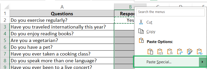
Step 4) From the Paste Special options, select Validation only.
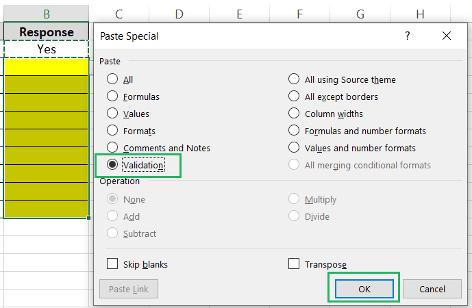
Step 5) Press okay.
This is how the drop-down list is pasted (note the yellow highlight remains in its place and the no-cell highlight formatting of the copied cell is not pasted). Only the drop-down list is pasted 💡
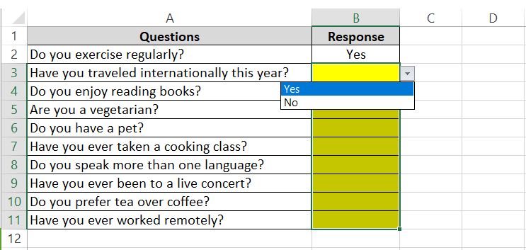
So, you get the drop-down list copied and pasted to as many cells as you want (can be anywhere in your sheet) and you do not even have to compromise the formatting of the destination cells.
This is something I call a win-win situation.
Edit the Yes or No options in Excel
Once you’ve created a drop-down list in Excel, to make any edits to it, you’ll have to edit the data validation rules by following the steps below.
Step 1) Select any of the cells where you’ve applied the data validation rules.
Step 2) Go to the Data tab > Data Tools > Data Validation.
Step 3) In the data validation box, make the desired changes.
Can be any changes, you might want to change Yes or No to True or False. Or for example, I am changing the No option to No! (With an exclamation mark) ❗
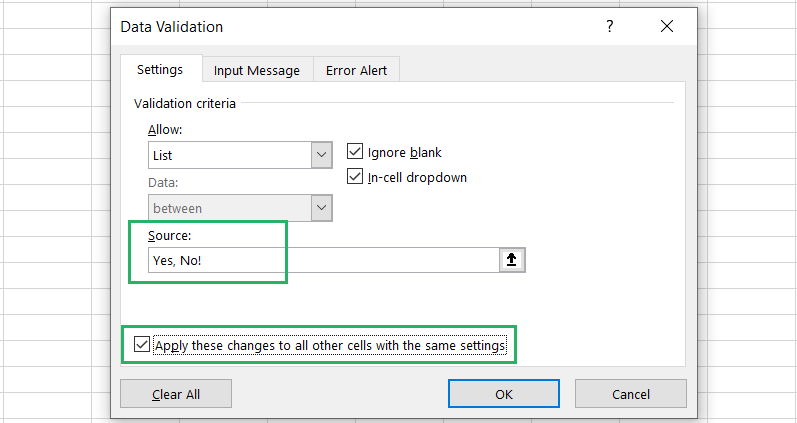
Step 4) Once done, check the “Apply these changes to all other cells with the same settings” check box.
Checking this option ensures the changes are applied to all the cells where this data validation is applied (if this is something you want; elsewise leave this box unchecked if you only want the change to apply to the selected cell).
Step 5) Click okay.
The change will be applied to all the cells and their drop-down lists.

By changing the original rule, you can change all the drop-down lists across your sheet.
If you’re going with method 2 (where the drop-down lists options are referred from other cells in your sheet), in that case, simply change the options in the cells where you originally wrote them.
The changes will be automatically reflected in all the drop-down lists based on them ✅
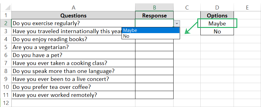
Easy!
Conclusion
Drop-down lists are an amazing feature of Excel.
They not only help you create a pre-defined list of values for the cells in your sheet so there’s nothing unwanted there, but they also help you save time.
If you want to create fillable sheets for circulation among users that are quick to fill with pre-defined options, what’s better than stipulating drop-down lists for each cell? This tutorial teaches how you can add yes or no options in your drop-down list in Excel (manually and through cell referencing).
Side Excel tips: we also saw cool ways to copy and paste it across other cells and edit it.
- To master the art of creating, editing, and removing drop-down lists in Excel, read the following Microsoft Excel tutorials by Spreadsheeto.
- How to Create a Drop-down List in Excel (in 60 Seconds)
- How to Edit a Drop-Down List in Excel (Best Methods)
- How to Remove a Drop-Down List in Excel (Step-by-Step)
