How to Create a Drop-down List in Excel
(in 60 Seconds)
An Excel drop-down list streamlines data input by making the user select text or values from a list of options, instead of typing them manually in a cell.
This enables you (the creator) to control all data entries for important cells.
The drop-down list is the most popular data validation tool in Microsoft Excel.
And it looks pretty cool too😎

Just follow these 5 steps and learn how to insert a drop-down list in Excel in 60 seconds (or less!).
Also, I cover how to control the input message and error alert.
If you want to follow along with how I create drop-down lists, download the free Excel worksheet here.
Step 1: Choose drop-down list items
Drop-down lists control data entry.
But before you insert the drop-down list you need to decide what data entries should be allowed. This is what we call the ‘list items’.
Pick anywhere you want to store the list of items for your drop-down list. It can be in the same sheet, another sheet, or in another workbook entirely.
Write the desired drop-down menu options in a list.
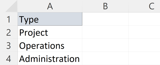
Step 2: Go to the ‘Data’ tab
This step is easy😊
Simply move your cursor to the ‘Data’ tab and left-click it.

Step 3: Click ‘Data Validation’
In the Data Tools group, click ‘Data validation’ in the middle of the ribbon.
(Do not click the little arrow – simply click the top part of the button).

Now, a dialog box called ‘Data validation’ appears. Here, you choose the settings for your drop-down list.
Let’s dive in🤿
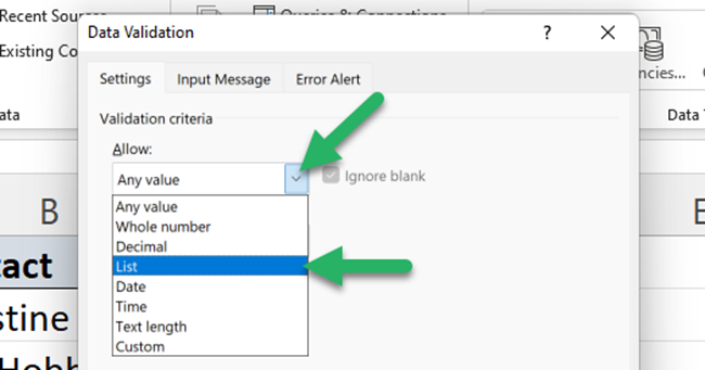
Step 4: Allow data validation ‘List’
In the data validation dialog box, in the Settings tab, click the drop-down list and pick what kind of data validation method you want to use (how meta is that?!).
Select ‘List’ from the… well… list!
I promised you could add a drop-down list in less than 60 seconds, didn’t I?
So, let’s keep up the pace🏃🏽
Step 5: Select the source list
Remember in step 1 where you chose the allowed options (list items) for your drop-down list?
Now it’s time to connect that list of options with the drop-down menu.
Left-click once in the ‘Source:’ box.
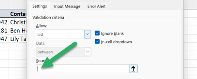
Then go to the location of your list with allowed values. The one you wrote in Step 1, remember?📝
Select the cells containing your drop-down list items.
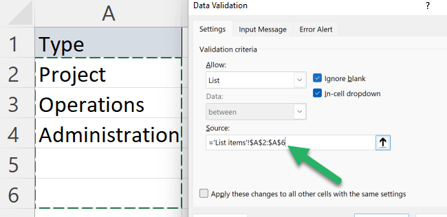
Click ‘OK’.
PRO TIP
As you can see from the picture above, I included a few empty cells at the bottom of the source range.
This allows not only for the addition but also for the ability to remove items from the drop-down list by deleting content from these cells.
Or, alternatively, I can write values directly in the “Source:” box, separated by a comma.
This is much easier than going back and changing the source range size every time new items are added.
It’s also much easier than creating a dynamic drop-down list, where the source range automatically adjusts to the data.
After you click ‘OK’ your drop-down list is ready for use.

Cool, huh?💪
Error alert
Using drop-down lists is primarily for selecting data entry instead of typing it manually.
However, the user can do manual data entry in the cell that contains the drop-down list.
But if invalid data is entered, an error alert will show.
The default error message doesn’t give a great indication of what the user can actually write in the cell.
To improve it, simply go to the ‘Error alert’ tab after opening the ‘Data validation’ window.
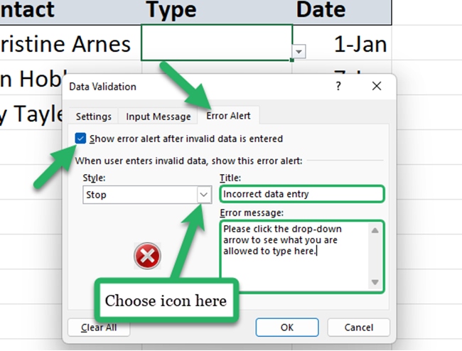
From here, make sure there’s a checkmark in the “Show error alert after invalid data is entered”.
Then, add the title and error message and choose an icon from the “Style” dropdown if you don’t like the default.
Then hit ‘OK’.
Now, this error message pops up whenever invalid data is entered into the cell.
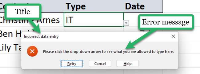
If you don’t check the “Show error alert after invalid data is entered” checkbox, anyone can write anything in the cell with the drop-down list.
Input message
Drop-down menus, and data validation in general, make it harder to input something wrong in your spreadsheet.
But the ‘Input message’ addition makes data entry even easier – and more bulletproof.
When creating a drop-down list, you can add an input message from the ‘Input message tab’ in the data validation dialog box.
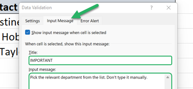
Simply type your input message and it will appear when the user selects the cell containing the drop-down list.
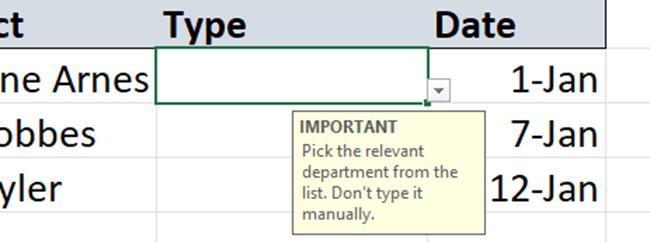
The input message is an easy way to improve the user experience of your spreadsheets – which is something most spreadsheet creators neglect.
That’s it – Now what?
You’ve just learned how to create a drop-down list in Excel.
Also, you can now control the error alert that is shown when invalid data is entered.
And you can make the spreadsheet show a nice input message to make the data entry process easier for the user.
Well done👍
But there’s more to Excel than eradicating typos with drop-down lists.
Let’s stop and think: Why are typos such a menace?
Because they make your functions less effective.
Especially the functions: IF, SUMIF, and VLOOKUP.
And they happen to be 3 of the most important functions in Excel.
If you’re not proficient with those already, I strongly suggest you enroll in my 3-part free online course and learn IF, SUMIF, and VLOOKUP once and for all.
Other relevant resources
Drop-down lists are part of a larger set of Excel features called ‘Data validation’. I’ve written the ultimate guide to data validation that teaches you everything you need to know. Check it out here.
I’ve also just written new tutorials that dive into how to remove drop-downs and how to edit drop-downs.
There are also a few ways of using drop-downs that cater to niche scenarios. For instance, you can make drop-down lists where the list items change depending on what the user picks in another drop-down list.
That’s called dependent drop-down lists (some call them cascading drop-down lists), and you can learn all about it in my YouTube video below!
Pretty cool, right? 😎
In general, drop-down lists are great when typos and other invalid data entries are very annoying.
Filters suffer greatly from typos. So do pivot tables and lookup functions such as VLOOKUP, INDEX MATCH, and XLOOKUP.
Thanks for reading👋
