How to Use an Array Formula in Excel (+Examples)

Array formula in Excel is an exceptional feature that allows you to manipulate and organize large sets of data easily into a single cell.

For instance, you would need multiple nested IFS of SUMIFS functions to find the sum of values in your sheet based on different conditions.

But by using an array function, you can do the same task with a single formula returning a single result. The only hurdle is array functions are difficult to master but worry no more 😎

In this tutorial, we will understand what an array formula is and how you can use it to its full potential. Download our sample workbook here to practice along.

Table of Contents

What is an array?

In simple terms, an array is a collection of items divided based on rows and columns. Most commonly we use two dimensions of the array 1D and 2D.

Think of it like a list containing different items. The items in the list can be anything, from alphabets to numbers to entire strings,

For example, if you were to select a row and write a formula as:

Then press the array shortcut or CSE keys, i.e., CTRL + SHIFT + ENTER, you will get values in different columns as:

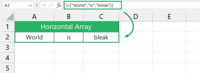
And you’ve successfully created a 1D horizontal array, That wasn’t difficult now, was it 😀

What is an array formula?

In simple words, an array formula in Excel allows you to perform multiple calculations on multiple cells in a range in one go. Its working is advanced as it can handle more complex calculations than a simple Excel formula would be able to.

You can use the array formula to return the result in either a single cell or multiple cells depending upon the nature of your task 🤔

This suggests, that an array formula inputs an array and returns a result corresponding to the array. It spills the values in neighbouring rows or columns.

Note that array formulas are accessible in all versions of Excel.

Understand this from a small example, suppose you have a data set of days in a month and you want to count, sum and find the average of the number of times each day appears.

If you were to do that using simple Excel formulas, you would have to find each result separately in three different cells. Using an array formula, you can do all that enclosed in one formula.

Let’s see a quick implementation of this example below.

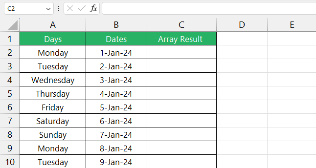
We have days and dates written out for January 2023 in the image above. Let’s now use our array formula to count, sum and average the occurrence of each day.

Type in the following formula in cell C2 and press Enter.

PS. Make sure to check for the curly brackets at start and end.

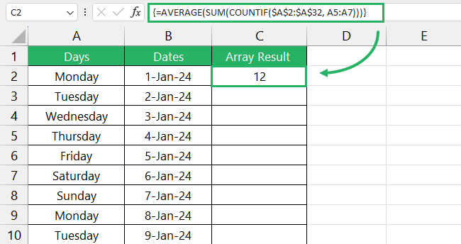
The formula returns the average of values from cell A5:A7 as 12 which is correct ✅

So instead of first calculating the count, then the sum and then the average separately, we saved ourselves the extra clicks and quickly got the average as a single result.

Imagine doing the same for a dataset containing hundreds of rows. That’s the efficiency array formula offers.

Pro Tip!

Don’t try entering the curly braces manually, it won’t work. And when you edit a formula, make sure to press CTRL + SHIFT + ENTER before saving the changes 💻

If you don’t use CSE keys, your formula will behave like a normal formula and will only take the first few values of the array as input.

What are single-cell and multi-cell array functions?

Single-cell and multi-cell array functions simply mean that they return the result of a formula in a single cell. If you select a range of cells where you want the values to be displayed, it would be referred to as a multi-cell array function.

Excel has a bunch of functions that return multi-cell results by default like the SEQUENCE, TRANSPOSE, RANDARRAY and other dynamic array formulas.

Let’s see an example for both single-cell and multi-cell array functions below 🔽

Single-cell array function

Suppose you have the following data set which contains the number of sales made for each fruit in two different months 📆

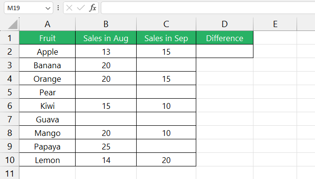
We want to count the number of sales made in each month and subtract them from each other to find the difference between the two.

Normally, to do the above task, you would first have to calculate the count of non-empty cells in two different columns and then find the difference.

We will do all this and return the result in a single cell using the following single-cell array formula.

Select a cell and copy and paste the following CSE formula.

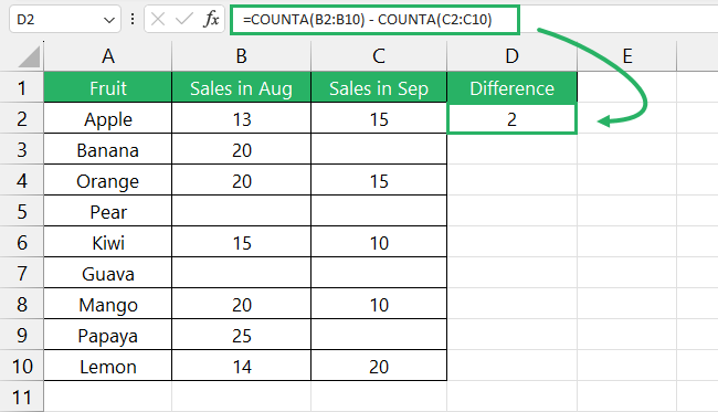
The array formula returns a single value 2, i.e., the difference between the count of values in both columns.

Multi-cell array function

Suppose you have a worksheet with amounts in USD to be converted to INR. Instead of converting each value, we will use a multi-cell array formula that will fill in all individual cells with their respective conversions.

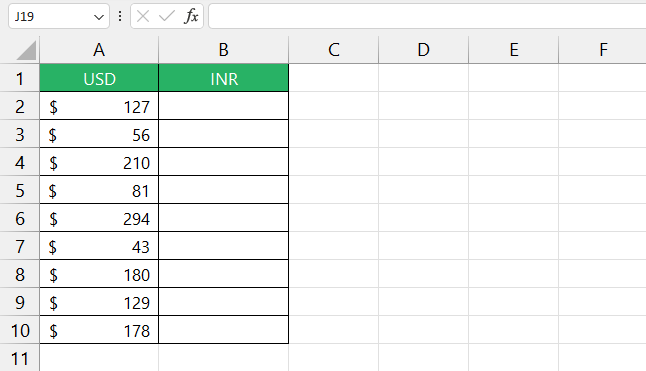
Select an empty range from B2:B10 and type in the following formula:

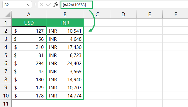
The array formula returns the converted currency in the selected range 🤓

How to break down an array formula?

Breaking down an array formula to see how each formula is evaluating a set of values and how the final result is coming together is very easy 🧐

All you need to do is select a formula and its arguments with a parenthesis and press the F9 key. If you wish to exit the formula breakdown, press the Esc key.

Let’s see it in the above example we used.

Without any selection, this is what the formula looks like in the formula bar:

Upon selecting the parenthesis, we press F9 and the formula turns into something like this:

The three 4 values here show the count of the values in cell A5:A7. You can do the same for the rest.

What are Excel array constants?

Array constants simply refer to an array containing items that do not change as you copy or paste values to other cells. We saw an example of this earlier in our tutorial.

Let’s learn more about them below.

Pro tip

Here are some key points you need to keep in mind when using array constants 🔑

Values in an array constant are separated either by commas or semicolons.

An array constant can contain boolean values, numbers in scientific, integer or decimal notations, and error values in an array constant.

You can include text strings but they must be enclosed in double quotes (““).

An array constant cannot hold formulas, ranges, other arrays, defined names, cell references or dates 📆

Types of array constants

There generally exist three types of array constants. These are horizontal, vertical and two-dimensional array constants 3️⃣

Horizontal array constant

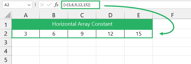
As the name suggests, a horizontal array constant refers to values printed in a single row.

For a horizontal array constant, you need to type the values separated by commas enclosed in braces (other than the CSE keys braces).

Step 1) Select a range in your spreadsheet where you want the values to appear.

Step 2) Type in the following formula.

Step 3) Press CTRL + SHIFT + ENTER on your keyboard.

Excel fills in the values in the horizontal array constant in selected cells as:

Vertical array constant

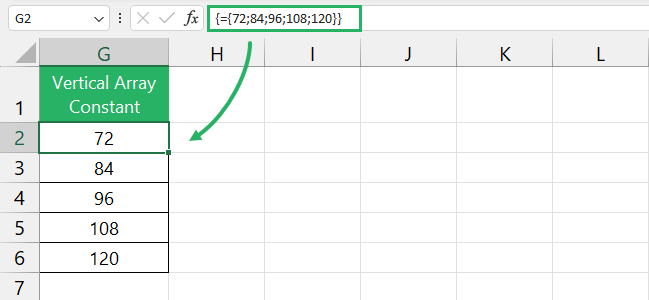
A vertical array constant is similar to a horizontal array constant. The only factor differentiating it is the separating character, i.e., semicolons.

Step 1) Select a range in your spreadsheet where you want the values to appear.

Step 2) Type in the following formula.

Step 3) Press CTRL + SHIFT + ENTER on your keyboard ⌨

Excel fills in the values in the array constant in selected cells as:

Two-dimensional array constant

A two-dimensional array takes in delimiters of both a horizontal array and a vertical array constant. You write the values separated by commas and semicolons.

Step 1) Select the range you want the values to appear in.

Step 2) Type in the following formula.

Step 3) Press CTRL + SHIFT + ENTER on your keyboard.

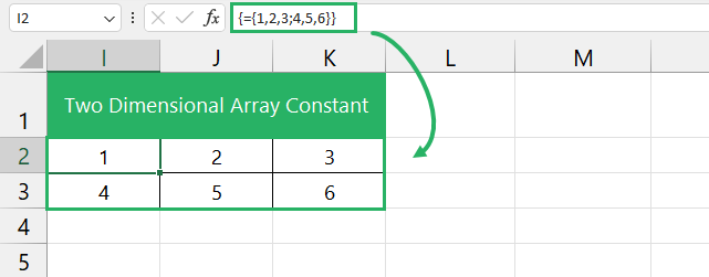
The values appear in two dimensional form in selected cells within no time 😀

Named array constants

An interesting feature Excel offers when using arrays is named array constants. You can give your array a name and use the name to print your array anywhere in your workbook instead of typing it.

To name your array constant,

Step 1) Go to the Formulas tab on the ribbon and under the defined Names section, click on Define Name.

Step 2) You can also use the CTRL + F3 shortcut followed by the New option to open the same.

Step 3) Once done, in the Name box, type in the array name.

Step 4) In the Refers to box, type in your array enclosed in braces with an equal sign at the beginning.

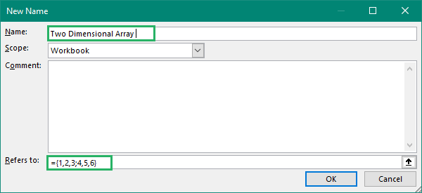
Step 5) Press Ok.

Your named array constant has now been saved ✔

To print the named array in your worksheet,

Step 6) Select the range of cells corresponding to your array size.

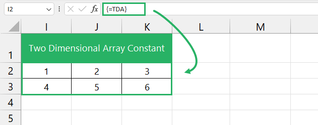
Step 7) Type in the name of the array preceded by the equal sign as:

Step 8) Press the CTRL + SHIFT + ENTER keys on your keyboard ⌨️

Excel will print your named array in the selected range

Debugging the array constant

If your array constant is not working as expected, here are some ways you can debug it 🧐

Check if you’ve used correct delimiting characters (commas for rows, semicolons for columns) in your array constant.

Make sure you select the exact number of cells as the items in your array. If you select cells less than the number of items, the array will only be partially displayed. If you select more cells, it will give a #N/A error in all remaining cells.

Unary operators in Excel array formulas

In Excel, we have two operators that tell the formula what logic you want to apply or how you want the arrays to be processed – the AND and the OR logic.

The AND operator uses the asterisk sign (*) which refers to multiplication and returns TRUE when all conditions in a formula are met.

The OR operator uses a plus sign (+) which refers to addition and returns TRUE when even a single condition in the formula evaluates to TRUE ✅

Let’s see an example of both operators with an array formula.

AND Operator

Say, we want to calculate the products of some numbers and sum their products as done here.

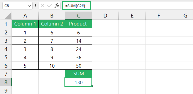
Now instead of filling two columns with values, applying the PRODUCT function and then the SUM function as done above, we can use simply use array constants in an array formula.

Not only will this make the entire calculation hassle-free but will also return the result in a single cell. To do this,

Step 1) Select a cell.

Step 2) Type in the following formula.

Step 3) Press the CSE keys.

The array formula will return the result:

It multiplies each element of the array with its corresponding element using an asterisk and then sums each product and returns the final value 😃

OR Operator

The OR operator works as suggested – it returns true when any one of the given conditions is being met. Let’s visualize this through an example.

Say, in the sample dataset, we want to count the number of scores in a list that are either greater than 80 or less than 60. For this, we will use an array formula coupled with the OR operator.

Step 1) Select a cell.

Step 2) Type in the following formula

Step 3) Press the CSE keys.

The array formula will return the result:

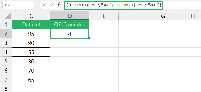
It gives the count of values that meet the conditions specified in the formula ➗

Conclusion

In this tutorial, we saw what an array formula is, how you can use it and some easy examples. Array formula is one of the best and most powerful features of Microsoft Excel 💪

You can use them to manipulate data spread over hundreds of rows easily. To read more about array formulas in Excel, check out the following links.

How to Use Multiple Formulas in a Cell (Excel Guide)

How to Use the SEQUENCE Formula in Excel (Easy)

We hope you enjoyed reading this article as much as we did crafting it 😃