How to Calculate Ratios in Excel
(Ratio Formula)
Past is a good place to visit so how about I take you back to elementary mathematics where we studied ratios?
Ratios express the quantitative relationship between two numbers that shows one number is how many times the other number.
For example, if you have a box with 8 red balls and 4 pink balls, what’s the ratio of red balls to pink balls? 🤔
It’s 2:1. This ratio means that for every 2 red balls in the box, there is 1 pink ball. Or you could say the ratio of red balls is twice that of pink balls which means you have double red balls than pink.
Ratios are super important, and you’d see them being used almost everywhere around you and this tutorial is all about calculating ratios in Microsoft Excel.
Download your free sample practice workbook for this guide here and let’s go spread sheeting!
Methods to Calculate Ratios in Excel
Ratios are often expressed as a fraction like a/b or percentages, but most commonly they are written as an expression with a colon in between (a:b).
There are no inbuilt Excel functions to calculate and express ratios in the above format.
But that’s alright – we have many methods to calculate ratios and express them in whatever format we like in Excel. Ready to explore them all? Let’s go 🚀
Basic Division + ROUND function
A ratio expresses one number as a proportion of another number. For example, what is the ratio of 20 and 5?
Divide 20 by 5 to know it’s 4 (or 4:1). Tells that you can calculate ratios very well by using basic division in Excel ➗
To calculate the ratios for the following set of numbers in Excel.
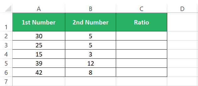
Step 1) In column C, write the basic formula for division as:
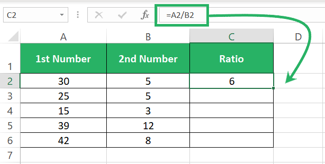
Tells you how many times the 1st Number is of the second.
By this result, we already know that 30 is 6 times greater than 5 (6:1).
Now to bring it in a:b format in Excel:
Step 2) Wrap the above formula as below and press enter:
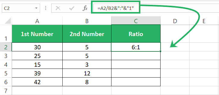
We just concatenated the results of the division function with a colon (:) and 1.
Step 3) Use the fill handle to drag and drop it to the whole list.
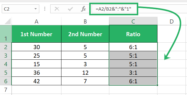
The above formula works fine for numbers like the above.
But just if we tweak the data to include numbers that are not very precisely divisible by each other (like below), the results might look a little clumsy 💨
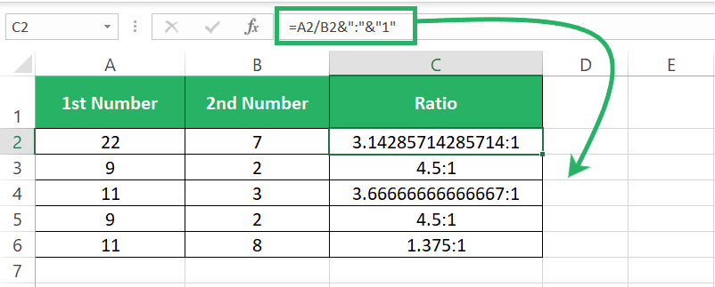
This is because some numbers when divided might result in multiple decimal positions or even recurring decimal positions making the result look like that.
But no problem. We will use the ROUND function to round the result to 1 decimal position (you can round it to any number of decimal places that is fine with you).
Step 4) Wrap the division formula in the ROUND function as here:
And now nest this function in the above formula in place of the division formula.
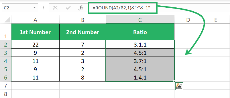
Aha! Looks much cleaner now 🧹
Using the GCD Function
GCD stands for Greatest Common Divisor – oh, even this phrase brings me back to reminiscences of my high school 👨🏫
The GCD function of Excel finds the greatest common divisor for any two given numbers (or more).
The process to find ratios in Excel using the GCD function is the same as above except for the difference that instead of dividing Number 1 by Number 2, we will divide both the numbers by their GCD.
Step 1) Write the GCD function for the following dataset as follows
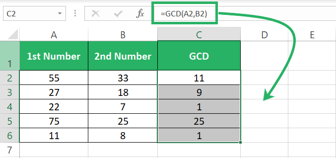
Calculate the GCD for all the numbers.
Step 2) To calculate the ratio, divide each number with its GCD and concatenate the results with a colon (:).
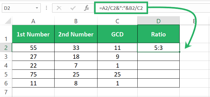
The above formula reads as:
First Number divided by GCD + concatenate + Colon sign (:) + concatenate + Second Number divided by GCD
The result gives a perfect whole-number ratio.
Step 3) Drag it down to the whole list.
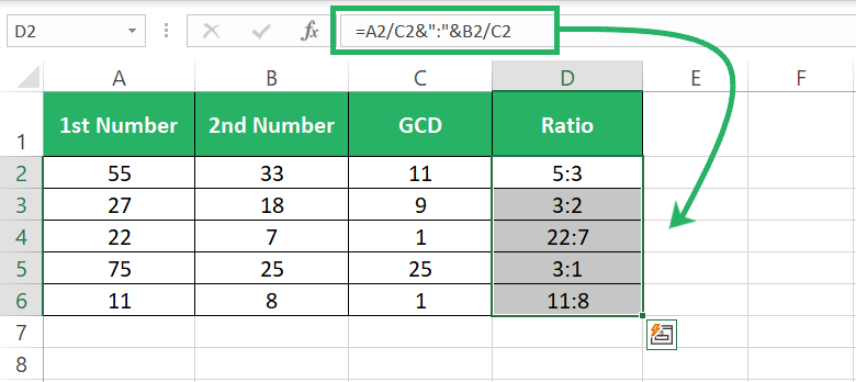
Here’s a quick check:
Since the numbers in this dataset are not divisible by each other, had we calculated their ratios using the simple division + ROUND function method, the results would have been very different.
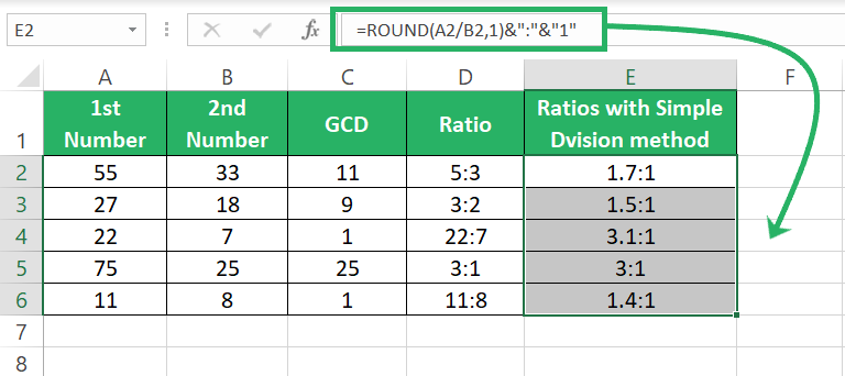
Hope this explains when you should use which method.
Using Text and Substitute Function
The next we have is the TEXT and SUBSTITUTE function. This one’s a little longer than the previous methods we’ve seen.
Let’s do it.
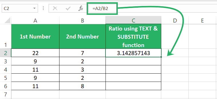
Step 1) Calculate the ratio by using a simple division formula as below.
Step 2) We will now nest the above function in the TEXT function to change the format of the results it has produced.
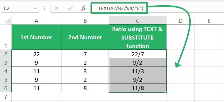
The TEXT function changes the format of a given value to any format you give.
So, we told the TEXT function to change the value A2/B2 produces to fraction format (##/##).
The answer until here i.e., 22/7 is also absolutely fine. Ratios are also expressed as a/b. But if you want it expressed as a:b, you will have to use the SUBSTITUTE function to substitute “/” with a colon “:”.
Step 3) Nest the above function in the SUBSTITUTE function as below.
Telling Excel to take the results of the TEXT function and from them, replace the “/” sign with a “:”.
And Excel rightly does so 😎
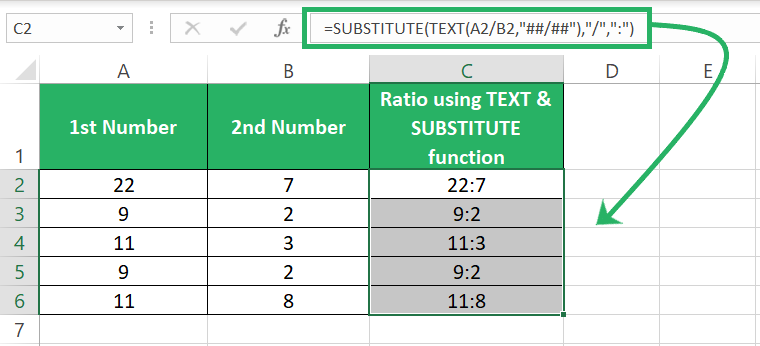
So, you have the ratios done.
Using Custom Fraction Format
If you don’t necessarily want the ratio to be expressed as a:b and if the a/b format works for you, you can achieve the above results without using the TEXT function. But only by applying a custom format to the results📝
Check this out.
Step 1) Calculate ratios by using a simple division formula as below.
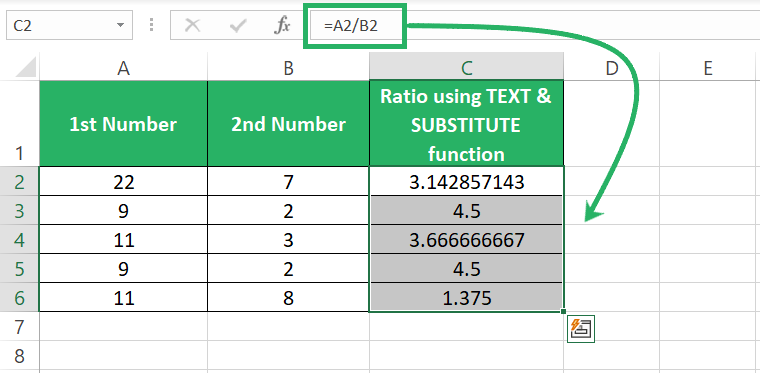
Step 2) Select the cells that contain the results.
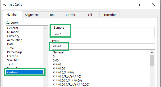
Step 3) Go to the Home Tab > Number group > Format.
Step 4) Go to More Formats
Step 5) Select Custom Format and type in the following format.
Step 6) Click okay and the results will look like this.
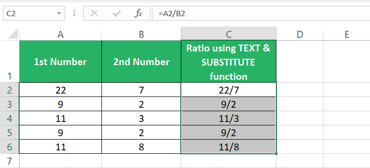
Note that this is only how the value is presented in the cell (fraction format). In the formula bar, the same division formula is running.
Using a VBA Code
And then, lastly, if you’re not in the mood to make a lot of effort or are running short on time to write formulas, just copy and paste this code into MS Excel and the rest will be done automatically 💻
Important!
To make this Excel VBA code work, make sure your numbers are in the worksheet named “Sheet 1”. Numbers should be populated in Column A and Column B of the said sheet (starting from Row 1). This code will calculate and populate the ratios in Column C.
To find ratios use this code:
Step 1) Copy the code below.
Step 2) Press the Alt key + F11 key to launch the VBA Editor in MS Excel.
Step 3) From the Ribbon on top, go to the Insert tab > Module.
Step 4) Paste the VBA code you copied above in this Module pane.
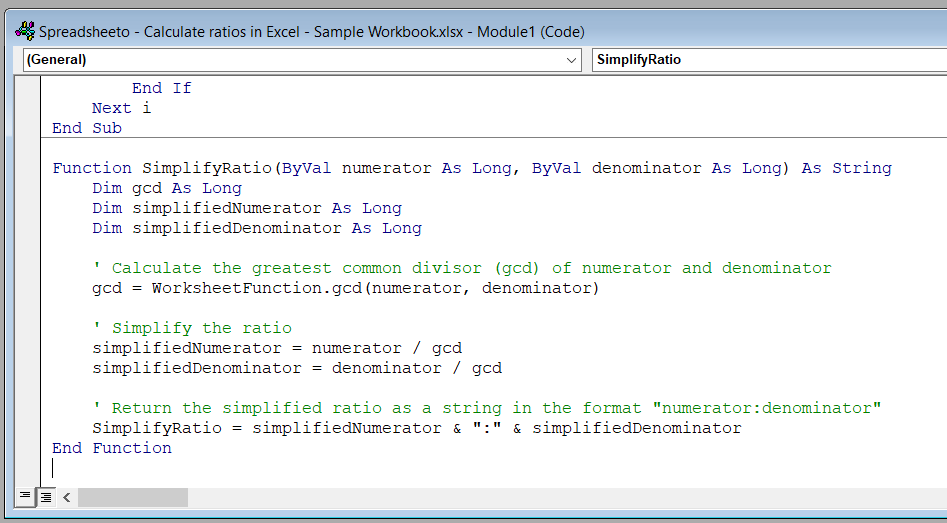
Step 5) Close the editor and press the Alt key together with the F8 key.
Step 6) Run the “ConvertToRatios” named Macro.
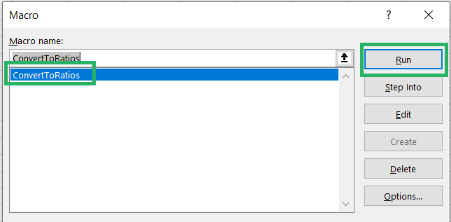
And magic! You get ratios for the numbers populated in Column A and Column B in Column C 🧙♀️
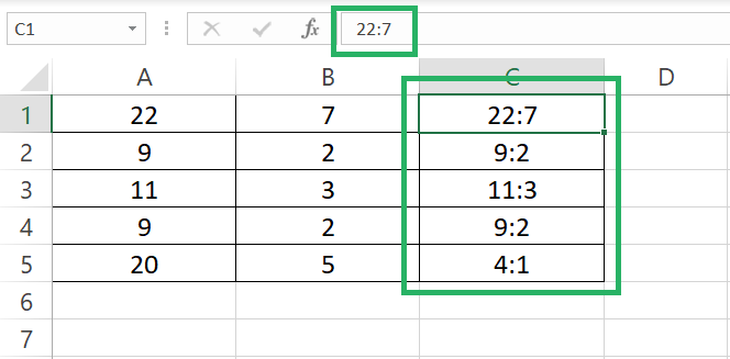
The result of this code will be just ratios in Text format with no formula running behind them. So, if you change any numbers later, the ratio will not update automatically. You’d have to re-run the code to get updated results.
Conclusion
The tutorial above covers a comprehensive list of methods that you can use to calculate and correctly express ratios in Excel.
Ratios are fundamental in making comparisons between two values. Or for seeing one value as a proportion of the other. You’ll see them being applied on a massive scale across so many fields including finance, accounts, and even sciences.
Once you’re done learning ratios, check out my Excel tutorial on creating pie charts and other kinds of charts in Excel to learn how can you visualize ratios in the form of charts.
