How to Get Cell Address in Excel (ADDRESS + CELL functions)
To obtain information about any cell in Excel, we have two functions: the CELL and the ADDRESS function.
Using these functions, you can get the address, the reference, the formula, the formatting (and much more) of a cell.
These are some of Excel’s most underrated functions, and it’s about time you learn why🤷♂️
So jump right into the guide below. And don’t forget to download our free sample workbook here as you scroll down.
Table of Contents
How to use the ADDRESS function
The Excel ADDRESS function returns the cell address for a given row number and column letter.
It has a large but simple syntax that reads as follows:
=ADDRESS(row_num, column_num, [abs_num], [a1], [sheet_text])
In order to address the first cell (Cell A1):
- Write the ADDRESS function as follows:
=ADDRESS(1,1)
- Hit Enter to reach the following result.

The first argument represents the row number (Row 1). The second argument represents the column number (Column 1). And so the resulting ADDRESS is $A$1.
That’s all that you need – the rest of the arguments are only optional ✌
- Now write the ADDRESS function with the third argument (abs_num) set to 4.
=ADDRESS(1,1,4)
- Press Enter and here are the results:

By adding 4 as the [abs_num] argument, Excel changes our result to a relative cell reference. Something completely different from what we saw earlier.
That’s because different values for the abs_num argument return different address types.
Pro Tip!
For the [abs_num] argument:
- If you enter 1, the address type will be an absolute cell reference ($A$1).
- If you enter 2, the address type will be a mixed cell reference. (A$1 – An absolute row reference, and a relative column reference).
- If you enter 3, the address type will be a mixed cell reference. ($A1 – An absolute column reference, and a relative row reference).
- If you enter 4, the address type will be a relative cell reference (A1).
In the first example, we omitted the abs_num argument and Excel set it to 1 by default. The result was, therefore, an absolute cell reference.
But the formula doesn’t just stop here🚀
- Include the fourth argument [a1] to modify this formula further.
=ADDRESS(1,1,4,0)

Here, 0 represents the reference style.
Note that the result is in a different style from our previous example. That’s because we opted for the R1C1 reference style in which columns and rows are represented by numbers.
- To get the result in A1 reference style, add 1 as the [a1] argument :
=ADDRESS(1,1,4,1)
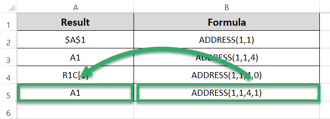
Note that we got the same result for our second example too.
That’s because if we omit the [a1] argument, Excel, by default, sets it to 1.
And what if you want the cell address from a different Excel sheet than the one you are currently on?
For this, you need to use the last optional argument of the ADDRESS function, i.e., [sheet_text].
It identifies the worksheet you want the cell address for 👀 Let’s try it out here:
- Write the [sheet_text] argument of the ADDRESS function as below:
=ADDRESS(1,1,4,1,”Sheet1″)
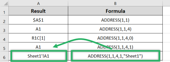
With the sheet_text argument as above, Excel generates an external reference. It returns the name of the worksheet with the cell address.
Like in the above example, Excel returns the address of the cell from Sheet 1. The Cell address is therefore prefixed by the worksheet name “Sheet1”.
If this argument is omitted, the resulting cell address won’t contain the worksheet name. And the address of the cell will be of the current sheet, by default.
How to use the CELL function
Until now we’ve seen how the ADDRESS function helps you find the address of a cell in Excel.
But what if you want to know about the location, format, formula, and content of a cell too🤔
The CELL function of Excel will help you fetch all these (and even other details about a cell). The syntax of this function reads as follows:
=CELL(info_type, [reference])
Starting with info_type, write the CELL function like this:
=CELL (
As you start writing the CELL function, Excel launches a drop-down menu of options for the argument “info_type“.
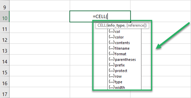
You can select from any of the 12 options in the drop-down menu above.
For example, select the option “Address” as the info_type argument. And Excel would return the address of the active (or the referred) cell.
= CELL (“Address”)
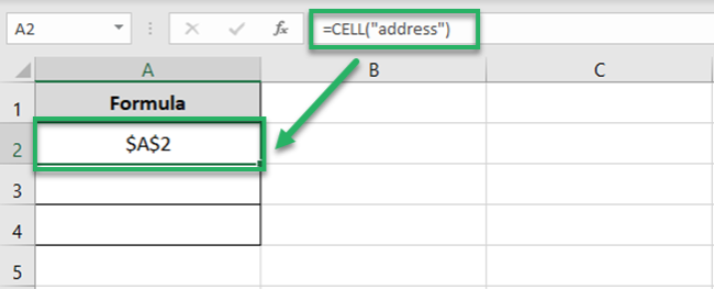
Note that we omitted the second argument of the CELL Function in the above example, i.e., [reference].
And so, the function returned the address of the active cell (Cell A2).
Pro Tip!
As the reference argument, you can refer to a single or a range of cells.
That’s not it – we still have 11 more info types to try and test.
So let’s change the arguments of our function as follows:
=CELL (“col”, A3)
Note that here we have created a reference to Cell A3 as the [reference] argument.

In this example, “col” represents the column number of cell A3 (the referred cell). The result given by Excel is 1 (the Column number for Cell A3).
Similarly, you can try different info_types to get different information about a cell. Like the following:
=CELL (“type”, A4)

“Type” returns the type of the referred cell.
Excel returned the value “B” indicating that the cell is blank. This is because we have referred to Cell A4 which is an empty string.
Pro Tip!
Under the “type” mode, if your cell contains a text constant, the result will be “I“. “B” if the cell is blank and “V” if the cell has any other data type.
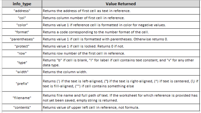
The CELL function offers a wide variety of info types that you might fetch for a cell. Here’s a short tabular summary of them all 👇
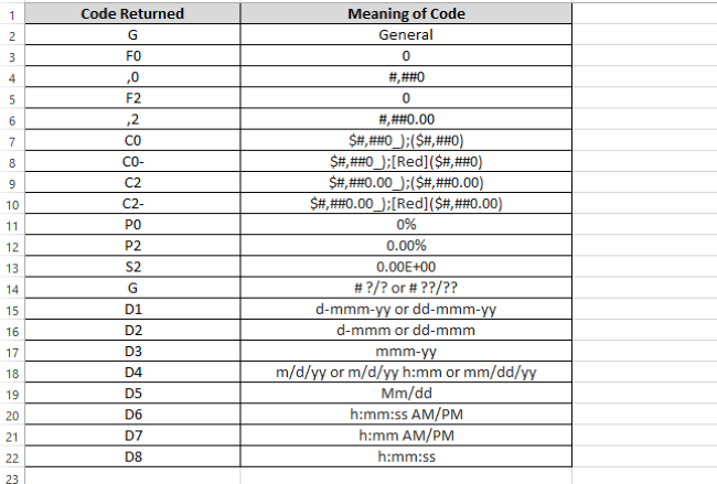
The format info_type returns the format of the referred cell. It gives different results for different cells which are in the form of codes.
The image below shows a list of some common format codes along with their meanings and results. This should help clear out any confusion 🔍
That’s it – Now what?
In the above guide, we learned how to use two of the least-known yet very useful functions of Excel – the CELL and the ADDRESS function.
Finding information about a cell is no more a difficult task – thanks to the CELL function.
The ADDRESS function is also an excellent tool when used the right way. But it’s not the only one. Excel has a wide variety of functions that are equally or even more useful💪
To mention a few, the VLOOKUP, SUMIF, and IF functions of Excel. Register for my 30-minute free email course to master these right away.
Other resources
If you enjoyed reading this article, we bet you’d love to read our other blogs too. There’s certainly a lot more to learn about cell addresses and references in Excel.
Like how to use the ROW function to find the row number in Excel. Or how to use the COLUMN function to find the column number in Excel.
