How to Change Legend Text & Name in Excel (Step-by-Step)

One of the many reasons why Excel outstands all other spreadsheet software is its excellent charts/graphs and other visual tools library.

You can not only store data in Excel but also create charts and graphs out of it in Excel (very quickly and easily) 📈

To make the best use of charts in Excel, you might want to edit some parts of it to make it understandable. One of these parts is the chart legend.

In this guide, we will learn how to change the legend text and name in Excel in under 2 minutes. Here’s you free practice workbook for this guide, download it now and read with me till the end.

Table of Contents

What is a legend?

Legend is a key that represents different elements of the data series.

It helps the users understand which part of the chart represents which data series. This makes reading and understanding the chart easy.

For example, below is the data for some monthly sales of 3 products;

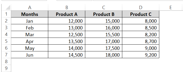
If I make a stacked bar chart out of it, it will look like 📊

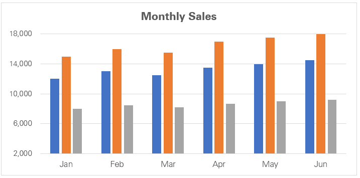
There are different colored bars in the chart, but which bar represents what? Barely makes sense.

If we add legends to it, the chart will begin to make a lot more sense.

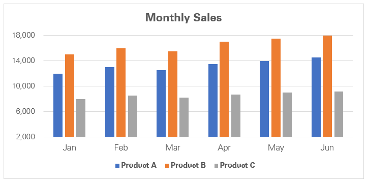
Legends are the small keys (which can be placed anywhere around the chart) that show which color/element represents what.

With this, we know that blue-colored represent the sales for Product A, orange-colored bars represent Product B, and grey-colored bars represent Product C.

Now, if I look at the sales for January, I can tell that the maximum sales were for Product B (tallest orange bar), then for Product A, and then Product C 📝

Hope this explains what legends are and why they are so important for charts and graphs interpretation.

Change Legend Text in Excel by changing the data

Whenever you create a chart with multiple categories in Excel, legends are added to it by default. The text for these legends is retrieved by Excel from the headers of the data.

Like in the above example, the legends are named Product A, Product B, and Product C. Excel has derived these names from the column headers of the underlying data 👀

Now, if you want to change the text of these names, one way is to change the source name from which they are derived.

Step 1) Identify the data headers from where Excel has derived the legend names.

This will not be challenging at all and most of the time, you will find these names readily placed before you in the dataset.

In our exemplary dataset, these are coming from these headers.

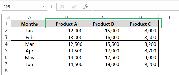
Step 2) Edit these headers to include whatever text you want for the legends.

For example, I want Product A, Product B, and Product C to be replaced by the product names (Refrigerator, LCD, and Heater, respectively) ✍

I will edit the header names accordingly.

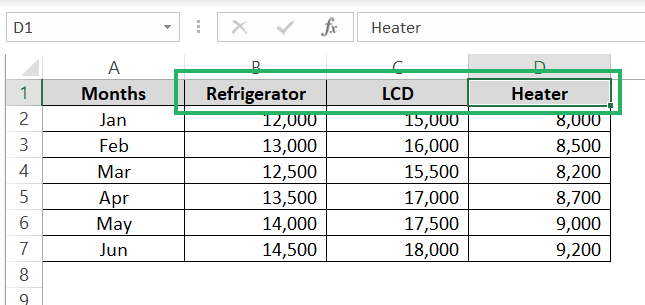
And as soon as I do that, the legends in the chart will update automatically.

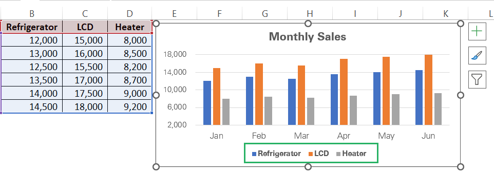
This is how you can edit the text of the legends by making changes to the data.

Change Legend Text in Excel from the Select Data tab

If you don’t want to make changes to the source data but still rename the legends, follow the steps below to update the legend text 🚀

Step 1) Select the chart by clicking anywhere on it.

Step 2) Go to the Chart Design tab on the Ribbon > Data group > Select Data.

This will launch the Select Data Source dialog box as below.

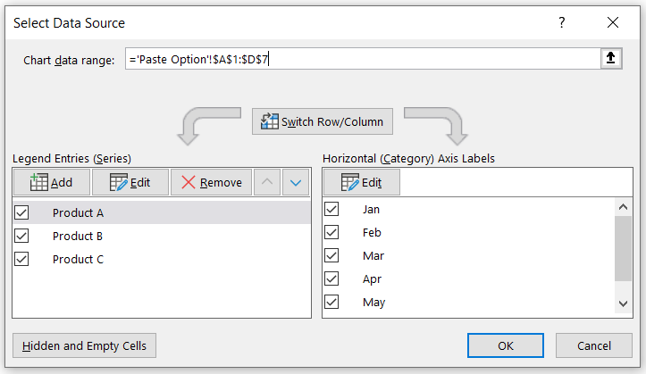
Step 3) Select the relevant legend (like I have selected product A).

Step 4) Click on the Edit button under Legend Entries.

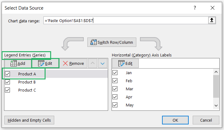
Step 5) Under the Edit Series dialog box > Series Name, define the text for the legends as desired.

For Product A’s legend, I will enter the new name as Refrigerator.

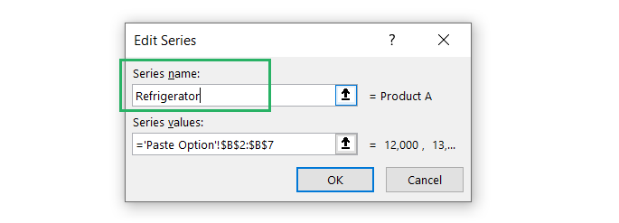
Step 6) Press okay under the Edit Series dialog box.

Repeat the steps above (from Step 3 onwards) for each of the remaining products (Product B and Product C) 📚

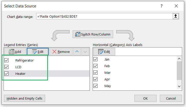
Step 7) Press okay for the Select Data Source dialog box.

And you’ll see the legends’ names will be changed.

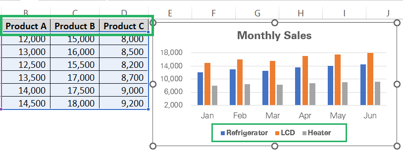
Although the legends are now named as Refrigerator, LCD, and Heater, the original data source remains unchanged with the headers as Product A, B, and C.

Conclusion

This guide discusses the two possible ways how you change can the legend text and name in Microsoft Excel by retaining the originality of the source data and by updating the source data.

You can choose whichever method suits you the best depending upon your need to preserve the source data 🗝

I have linked some other Spreadsheeto blogs below for you to check out to learn how to create a stacked bar chart and many other chart types in Excel.

• List of All Excel Charts & How to Use Them (2024 Tutorial)
• How to Create a Clustered Column Chart in Excel (+Stacked)
• How to Make & Use a Pie Chart in Excel (Step-by-Step)