How to Color Cells in Excel (Many Examples Explained)
Coloring cells in Excel is an everyday task and can improve the readability and visual appeal of your worksheet immensely.
Excel offers a variety of methods to color cells as you want, whether you want to color a row based on some rule or simply highlight an important column, you can do that in no time 🖌
In this tutorial, we will explore all the ways you can use to color cells in Excel. Download our sample workbook here so you can get on painting with us 🎨
Color cells in Excel manually
The most common method is to manually color cells using the Fill option. It can get slightly time-consuming if you have to apply different colors to different cells but works pretty well.
Say, we have the following sample data where we want to color the first five rows in red color and the last five in green color 🟩
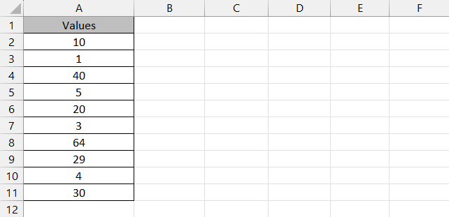
To do that,
Step 1) Select the rows you want to highlight.
Step 2) Right-click the rows.
Step 3) Select the Format Cells option from the dropdown list.

Step 4) In the Format Cells dialog box, go to the Fill tab.
Step 5) Select the color you want to apply to your cells.
Step 6) Click Ok.
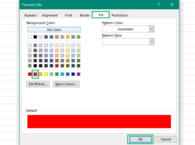
Alternatively, you can use an easier way to approach the same solution.
Step 7) Select the cells in your data set.
Step 8) Go to the Home tab on the ribbon and click on the down arrow next to the paint bucket icon in the Font group.

Step 9) Select the background color you want to apply to your cells.
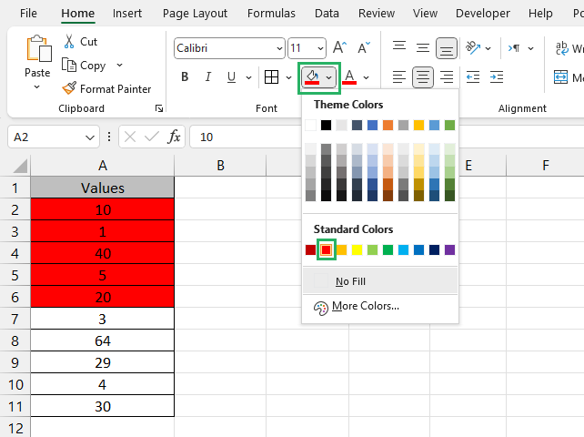
Step 10) Select the remaining half of your data set and repeat the process.
And it’s done.
All selected cells get highlighted in the chosen color:
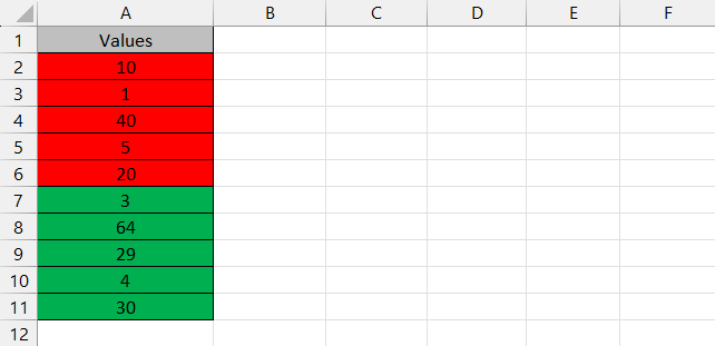
Pretty cool, no? 🤓
Color cells in Excel using Format Painter
Another way you can color cells in Excel is by using Format Painter. This is helpful when you have a large data set and you just want to format values copying from one place to the other ©
Format painter essentially copies the format of a cell and paints it to another cell. This means if your selection cell was colored yellow and had gridlines, for instance, the next cell you click will have the same format pasted to it but not the cell value.
We will use the same sample data as above. In this example, we will copy the color of the first five rows and apply it to the rows beneath them.
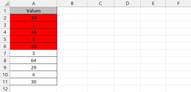
To do that,
Step 1) Select any cell from column A or row 2.
Step 2) Go to the Home tab and click on the Format Painter button in the Clipboard group.

Step 3) Click on the button and the format will be copied.
Step 4) Now select the rows beneath.
And it’s done! The format has been pasted to the selected rows as:
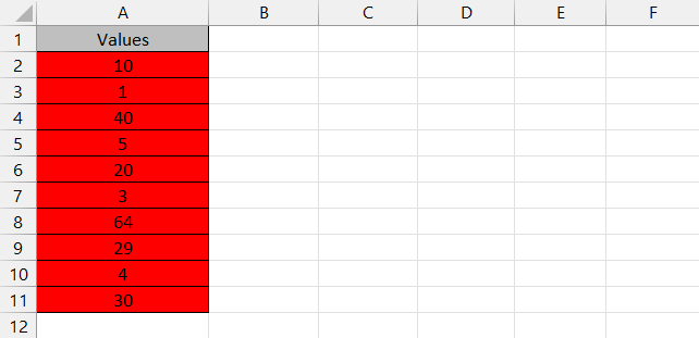
That was easy, no? 😉
Color cells in Excel using Find & Replace
You can also color cells using the Find & replace feature. This works best when you want to change cell color or want to color cells with the same content in one go 🥇
We will use the same sample data as earlier. We want to color all the cells in your data set that contain the value 10.
To do that,
Step 1) Go to the Home tab and select the Find & Select option in the Editing group or press CTRL + H to open the Find and Replace dialog box.
Step 2) In the Find What bar, type in your cell value.
Step 3) In the Replace with box, click on the Format button and select the color you want to be set.
Step 4) Press Ok.
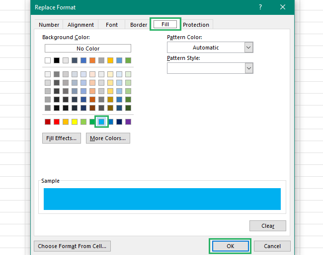
Step 5) Press Replace all.
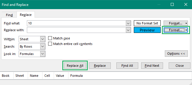
All the cells with value 10 have been formatted with blue color.
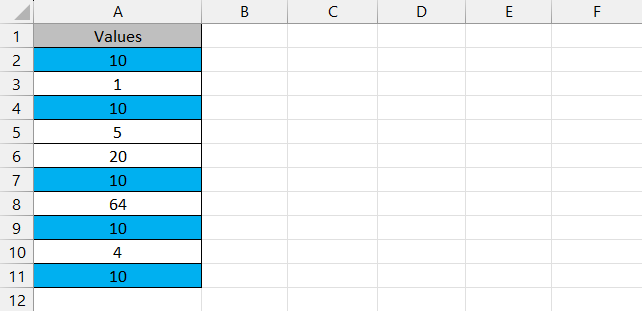
Try it now! 😀
Color cells in Excel using Conditional Formatting
Conditional formatting is slightly advanced when it comes to coloring cells in Excel but it offers a huge variety of ways you can choose to highlight cells 🖼
Excel conditional formatting is a powerful feature that lets you create your own rules for certain things. It lets you set the color of a cell depending on a condition and you can choose that condition.
We will use the same sample data as earlier. We want to color all cells in our data set red that have a value greater than 5 using a conditional formatting rule.
To do that,
Step 1) Select your data set.
Step 2) Go to the Home tab and select the Conditional Formatting option in the Styles group.
Step 3) Select Highlight Cell Rules or Top/Bottom rule type and select the condition you want to apply. You can create a new rule by clicking on the New Rule option. We chose the Greater Than option 💪
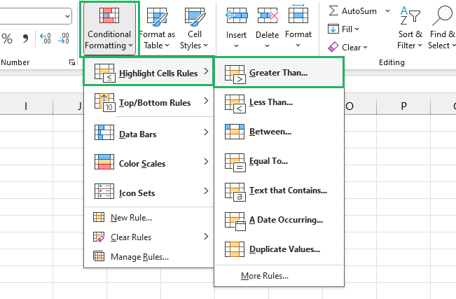
Step 4) The Greater Than dialog box appears.
Step 5) Enter the number for your condition to be valid and select the color format – we set it equal to 5.
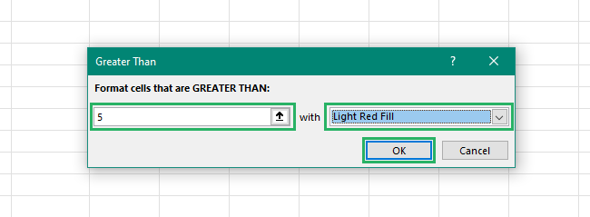
Step 6) Press Ok.
The range of cells selected will now be colored according to the condition:
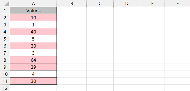
If you want to use a formula to format your cells, use the New Rule option. Select “Use a formula to determine which cells to format” and enter any Excel formulas you want to apply.
Color cells in Excel using VBA
Another way to color cells is using VBA where you create your own macro to perform a certain task. Let’s see how VBA works and how you can use it to your benefit 😎
The code below colors the cells in your given range green if they are below 20 and red if they are above 20.
To do this,
Step 1) Press Alt + F11 on your keyboard to open the visual basic editor.
Step 2) From the Insert tab, select Module.

Step 3) Copy the above code and paste it into the window that appears and close the editor.
Step 4) Press Alt + F8 on your keyboard to open Macros.
Step 5) Select ColorCells and press Run.
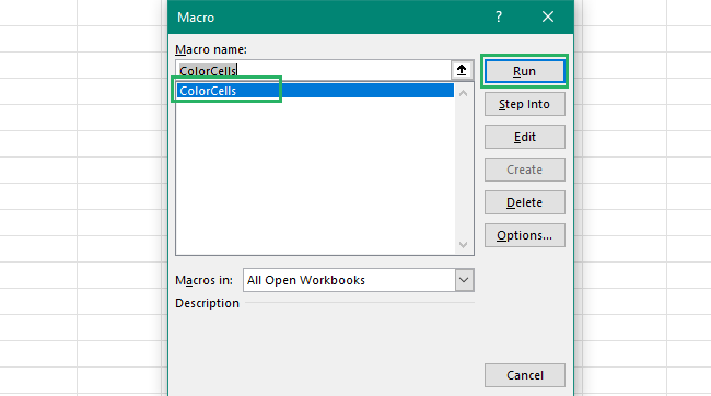
Step 6) The cells in your range meeting the condition will be colored as:
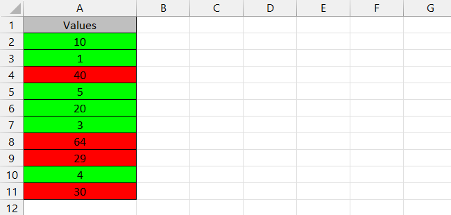
Pretty cool, right? 🧐
Conclusion
In this guide, we saw how to color cells in Microsoft Excel. We saw different ways including coloring cells manually, using Format Painter, find & replace and conditional formatting 🎨
We also saw how to highlight rows and columns using VBA in no time. To learn more about VBs, read our articles here.
Learn VBA in Excel: These 11+ Tutorials Teach You VBA in 20 Hours
How to Use Conditional Formatting to Highlight Text in Excel
How to Fill Color in Excel Cell Using a Formula
We hope you enjoyed reading this article as much as we did creating it 🤗
