How to Fill Color in Excel Cell Using a Formula

One of the core objectives of Excel spreadsheets is to increase readability and help data visualization.

And what helps data visualization better than eye-catching colors? Instead of scanning through large datasets, coloring them per your needs can shrink your data analysis time to less than half.

This can be achieved by using conditional formatting. The conditional formatting tool of Microsoft Excel allows you to certain formatting to be applied to cells if they meet the specified conditions given in the form of formulas 🎯

Believe me – all of this makes much more sense when practically applied. So, what are we waiting for? Grab your free practice workbook for this guide now and jump in straight.

Table of Contents

Why apply conditional formatting

There are many reasons why I’d vote for applying conditional formatting to cells to fill them with distinctive colors 😎

• Conditional formatting allows you to visually highlight important data points based on specific conditions. It helps in identifying trends, outliers, and other important data points at a glance.
• You can quickly pick out patterns or anomalies in your data without having to manually scan through large datasets. Saves time and facilitates informed decisions.
• Highlighting cells with different colors based on certain conditions improves the readability of data making it easier to interpret and understand complex datasets.
• Conditional formatting automatically updates the formatting of cells as the data changes.

Enough reasons, I guess. Let’s now see how you can fill color in cells based on a formula.

Applying Conditional Formatting to Cells

Time we see how you can apply conditional formatting in Excel based on some conditions/formulas.

I have a list of students together with their marks in a recent exam (out of 100) 👩‍🏫

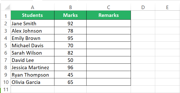
Here is how I want to remark on this score:

• Marks above 80: Good
• Marks above 50: Average
• Marks equal to or less than 50: Fail

Step 1) Write the IF function to have the Remarks automatically populated.

Step 2) Drag this formula down to the whole list of students.

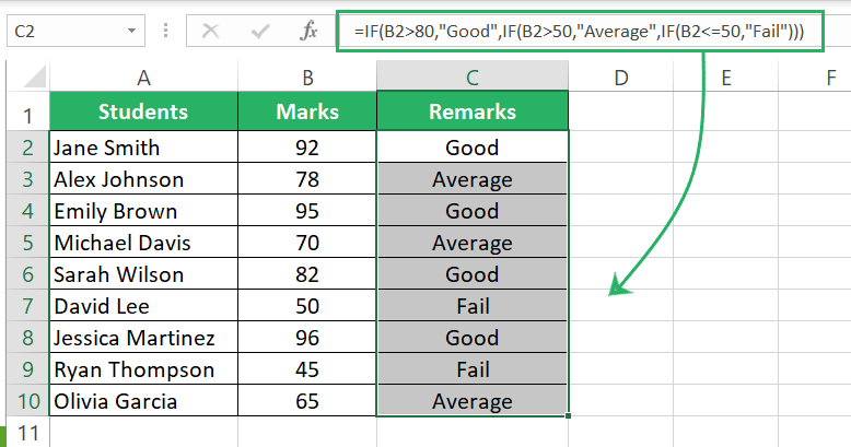
Excel automatically populates the remarks for students based on their scores.

Now, to conditionally format them based on these marks and the above rules, follow the steps below.

Step 3) Select the cells that contain the remarks.

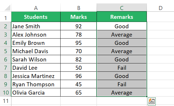
Step 4) Go to the Home tab > Style group > Conditional Formatting.

Step 5) From the drop-down menu, select Highlight Cells > Text that Contains.

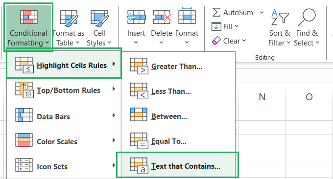
You will see the Text That Contains dialog box.

Step 6) In the text box, write Good and then select the format you want applied to it. Since it is a positive remark, I have set the format type to green highlight and text.

Excel shows a quick preview of how cells will be formatted and how they will look before the formatting is applied 💚

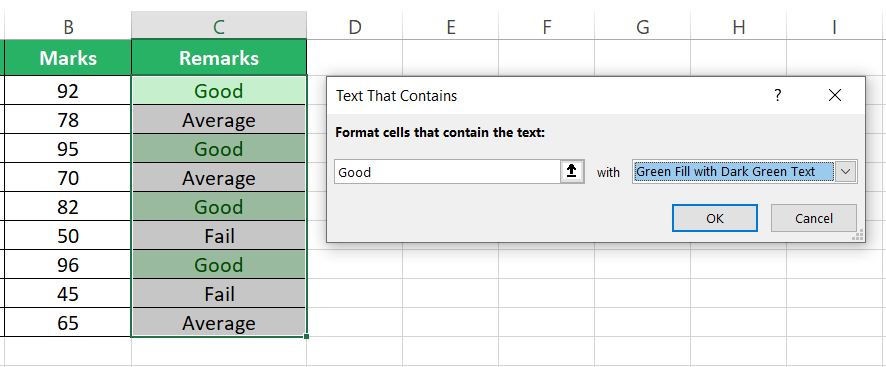
Step 7) Click okay, and Excel will highlight all the cells that contain the text “Good” in green.

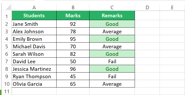
Step 8) Again, launch the conditional formatting rule for “Text that contains” following the steps as above.

Step 9) In the text box, write Average and select the format you want applied to it. I have set it to yellow highlight.

Check out the preview here 💛

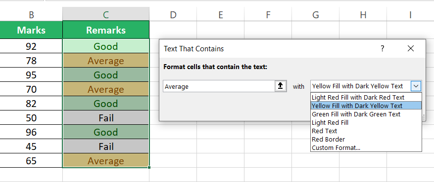
Step 10) Click okay to have the formatting applied.

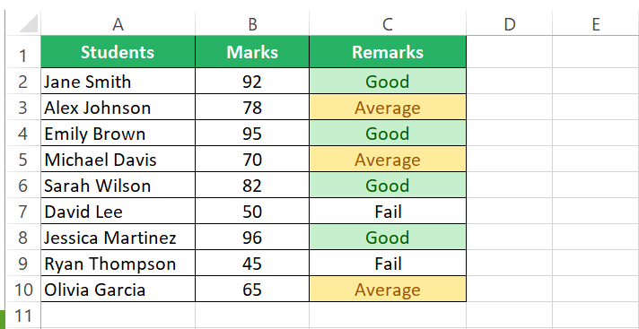
See how it works? Based on the condition that it contains the text “Average”, Excel highlights the cells yellow.

Step 11) Once again launch the “Text that contains” box.

Step 12) This time, in the text box, write “Fail” and select the format you want applied to it. I have set it to red highlight (well-deserved hype).

Here’s what the preview looks like.

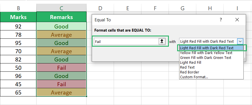
Step 13) Click okay, and all the cells that contain “Fail” will go alarming red 🔴

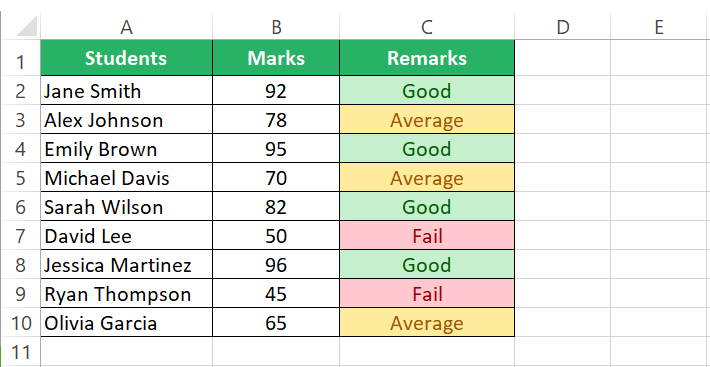
Wow! The data instantly looks so readable. Takes me a glance to identify the two students who failed.

And the 4 students who performed well are also equally prominent.

The best part: if any data changes, based on the rules specified, excel will automatically update the formatting for it.

For example, presently David appears to have 50 marks and is remarked as “Fail” (highlighted in red).

If I change his marks from 50 to 91, his remarks will automatically be changed to good (as they fall in the >80 categories), and accordingly, the formatting for his remarks will also change to “Green”.

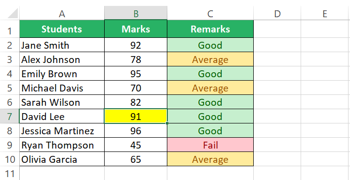
This was one way to highlight cells based on the text they contain.

We could also have done this by highlighting the marks based on the same rules on which they are remarked.

To do this, let’s revise the rules that we want to apply:

• Marks above 80: Good
• Marks above 50: Average
• Marks equal to or less than 50: Fail

Let’s apply them by beginning with the last rule.

Step 1) Select the cells in column B that contain the numbers.

Step 2) Go to the Home Tab > Conditional Formatting > Highlight Cells > Less than.

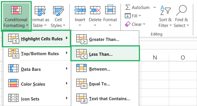
In the ‘Less than” dialog box, write 50 and set the format as Red highlighted (since we want the students who scored marks less than 50 to be considered as Fail and highlighted in red).

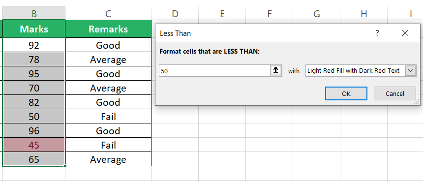
Step 3) All scores under 50 will be highlighted in red.

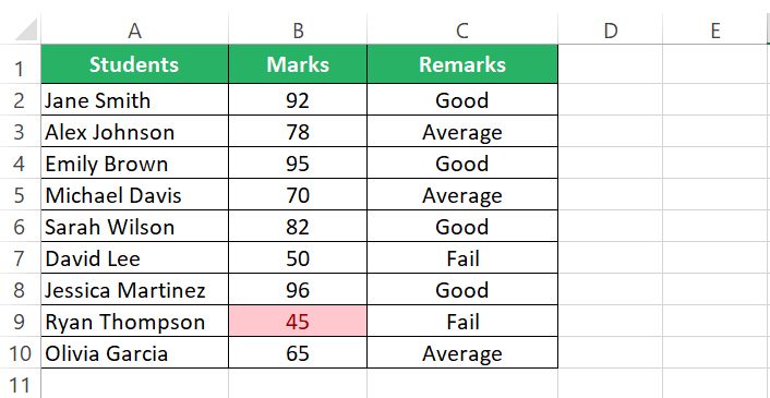
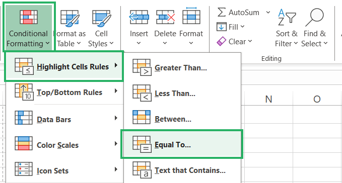
We have applied the rule for students who scored less than 50, let’s apply the same for those who scored marks equal to 50 📝

Step 4) Go to the Home Tab > Conditional Formatting > Highlight Cells > Equal to.

In the ‘Equal to” dialog box, write 50 and set the format as Red highlighted.

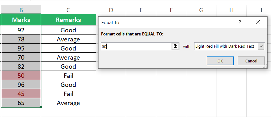
Step 5) All scores equal to 50 will also be highlighted in red.

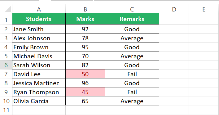
Huff! Done with the last rule. Let’s now move to the second last rule.

Step 6) To apply the second rule, go to the Home Tab > Conditional Formatting > Highlight Cells > Greater than.

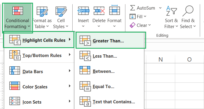
In the “Greater than” dialog box, write 50 and set the format as Yellow highlighted.

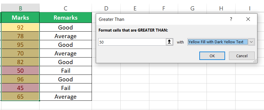
Step 7) All scores greater than 50 will also be highlighted in Yellow.

Pro Tip!

At this point, you’ll see even those scores are yellow highlighted that are greater than 80 (although we want them highlighted in green). This is because what’s greater than 80 is also greater than 80.

And this is alright – we will specify another rule for scores greater than 80 and this will be fixed. Conditional formatting works in the mode that the latest rule overpowers the previous one.

This is why we started applying rules from last to first (from the smallest score to the largest).

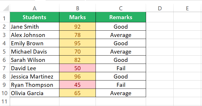
Step 8) Coming down to the first rule, go to the Home Tab > Conditional Formatting > Highlight Cells > Greater than.

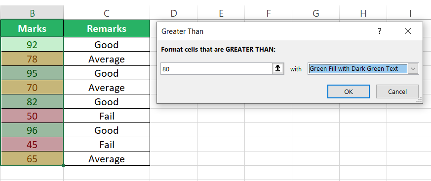
In the “Greater than” dialog box, write 80 and set the format as Green highlighted.

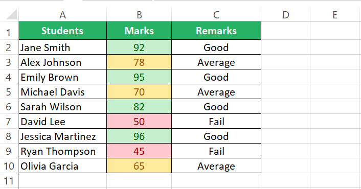
Step 9) All scores greater than 80 will now be highlighted in Green.

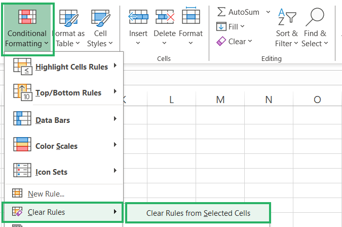
This sorts out all the scores and formats them based on their values and the rules set up by us. You can do it for text values and numbers.

I find using ready-made rules to format cells an easier way to conditionally format them. But these rules can only cater to certain and limited circumstances.

To take your conditional formatting to the next level, you can set up formulas as well.

For instance, if I want to highlight the name of the students who score equal to or less than 50, I’d have to set up a formula since the values that will be formatted (the student names) and the values based on which they will be highlighted (the students’ scores) are different.

Here’s how you do it:

Step 1) Select the names of the students.

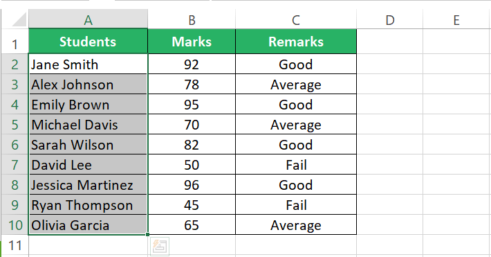
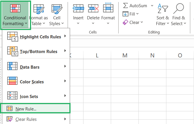
Step 2) Go to the Home tab > Conditional formatting > New Rules.

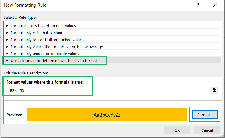
Step 3) In the New Rule dialog box, select the option “Use a formula to determine which cells to format”.

Step 4) In the Rule Description, write the following formula:

Comment

Make sure to use the exact same formula as above. B2 should not be an absolute reference but a relative reference. And the “less than” sign should come before the “equal to” sign in <=50.

Otherwise, you’ll not get the desired results.

Step 5) Set up the formatting that you want applied by clicking on the Format button.

Step 6) Click on the Okay button.

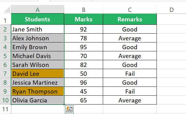
David and Ryan are highlighted orange since they scored less than 50.

Hope you enjoyed the versatility of Excel’s conditional formatting.

Conclusion

Conditional formatting is just an amazing feature of Excel. Leaves me in awe every time I use it.

You can write up any condition, or any formula, and Excel will highlight cells within any color and any format automatically. This cool tool of Excel has so much more about it to learn that you must not miss out on.

Here are some of my Excel tutorials that are highly recommended to be read for a better grasp of this and other tools of MS Excel.

• How to Use Conditional Formatting to Highlight Text in Excel
• How to Count Cells With Specific Text Using a Formula