How to Highlight Every Other Row in Excel: Step-by-Step
Highlighting every other (or alternate) row helps readability. Often when you have a pack of data with so many rows and columns, it gets hard to decipher the data.
So how can you highlight rows in Excel? Manually? Yes, you can do that, but only if your data goes across tens of rows (maybe).
But if your dataset extends to thousands of rows – this is an arduous task you’d never want to do 🙈
In the guide below, I am going to walk you through two smart (and automatic) ways of highlighting rows in Excel. You’d find them interesting, I bet.
So download the sample workbook for this guide here and dive right in.
Table of Contents
Highlight every other row with conditional formatting
Here’s the first method to highlight rows in Excel – by using conditional formatting 🎨
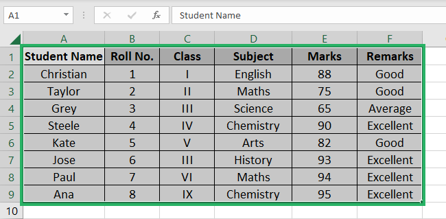
The image below shows a dataset with multiple rows (don’t mind the details).

We are on a mission to highlight alternate rows from this dataset using conditional formatting.
So here we go 🚴♀️
- Select the dataset where you want the conditional formatting applied.
If it is to be applied to the whole worksheet, select the entire sheet by pressing the Control key + A.
Pro Tip!
Leave out the headers (if your dataset has any) if you don’t want them to be highlighted too.
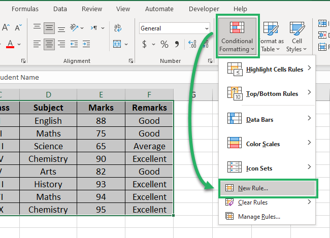
- Go to the Home Tab > Conditional Formatting > New Rule.
This takes you to the “New Formatting Rule” window as follows 🚪

Conditional formatting needs a condition to apply to the format. This condition can be supplied by creating a logical formula. Just like we will do now.
- Under Select, the Rule Type box, select Use a formula to determine which cells to format.
- In Edit the Rule Description box, write in the following formula.
= MOD ( ROW (), 2 ) = 0

Pro Tip!
What does this formula mean?
- The ROW function returns the row number for the cell (where you have written it). So for example, if you write the ROW function like = ROW () in Cell A2, the result would be 2.
- The MOD function divides two given numbers and returns any remainder. For example, if we write = MOD (5,2) the answer would be 1. Because 5 is not completely divisible by 2. Two times 2 is 4, and 5 less 4 is 1.
So by writing MOD ( ROW (), 2 ) = 0, we are dividing each row number by 2 to see if we get a remainder or not. This way all even rows will be highlighted 🔔
For example:
- MOD ( ROW(2), 2 ) answers 0. So conditional formatting tool will highlight Row 2.
- MOD ( ROW(3), 2 ) answers 1. So conditional formatting tool will not highlight Row 3.
- MOD ( ROW (4), 2 ) answers 0. So conditional formatting tool will highlight Row 4.
- MOD ( ROW(5), 2 ) answers 1. So conditional formatting tool will not highlight Row 5.
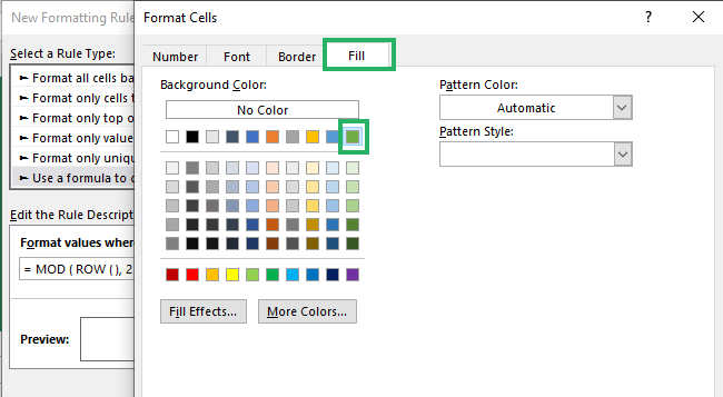
- Next, go to “Format” to select the highlighting color 😍

- Go to the Format tab > Fill.
- Choose the color to highlight the rows. We are selecting an earthly green color for now.
- Click Okay. And Tada 🌍
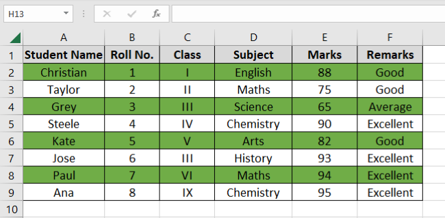
We have alternate rows highlighted in Excel. You must have found this way pretty straightforward, didn’t you?
Pro Tip!
As we move forward toward the next method of highlighting rows in Excel, must note the following 👇
Highlighting alternate rows using conditional formatting keeps the formatting intact even when you make changes to the data. For example, applying filters, sorting data, and adding or deleting data.
Highlight every other row with a table-style
Coming to the next method of highlighting alternate rows in Excel. This is more like an in-built method how you can highlight rows in Excel 📫
So here’s our dataset.

Right now, this is simply some data populated in Excel. Let’s convert it into a table.
- Select the data.
- Go to the Insert tab > Table.

This brings you the Create table dialog box as below.
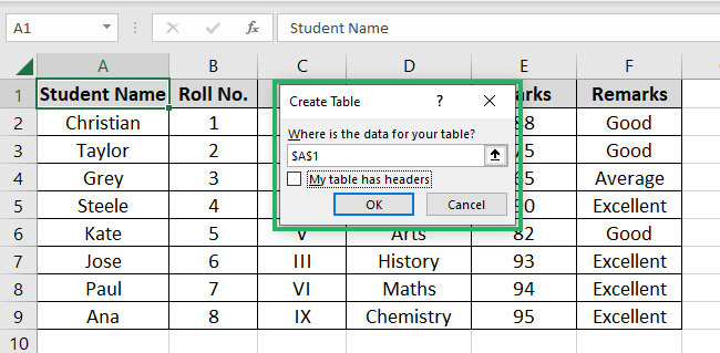
- Check the option for ‘My data has headers’ if you have selected the headers too 🎓
- Press Okay.

And your data is converted into a table. Yay!
Excel turns all the alternate rows into highlighted rows, by default. But if you want a different color applied, that’s still alright. Here’s how you can choose a custom table style.
- Select the table.
- Go to the Table Design > Table Styles > Drop-down menu icon.
Here’s a huge list of table designs 📃

- Select any of these (as desired). How about this?
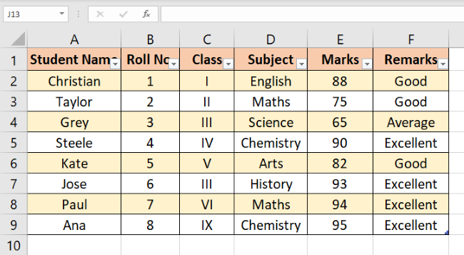
Play around with different styles to see if any of them fits your taste!
That’s it – Now what?
So we have come across two startling ways of highlighting alternate rows in Excel. Both are convenient, and easy and will save you hours of work time ⏳
Excel is a versatile spreadsheet program. Even if at some point, it fails to offer a particular feature, you’d be able to reach out a way to perform it by using Excel functions.
Talking about Excel functions – there’s a variety of them. And to become an Excel expert, you must know them all.
To start with, we suggest you go with the VLOOKUP, SUMIF, and IF functions of Excel. Want to learn them already?
Enroll in my 30-minute free email course that will help you learn them all (and much more).
Other resources
Want to know more about conditional formatting in Excel? Our guide will take you through it.
And why only conditional formatting? Hop on here to learn about the ROW and MOD functions of Excel too.
