How to Find and Remove Duplicates in Excel (Easily)
In an Excel spreadsheet, you’d often have to collate data from multiple sources. Sometimes from external sources (like webpages) too 🖨
And this might result in duplicates in your Excel sheet. So how can you remove them? By scanning your worksheet for dupes manually?
Nah! That’s not going to work if you have a large dataset. Let’s think of a smarter solution 🧠
To find and remove duplicate values in Excel, you can use the Remove Duplicate tool of Excel (and some other easy ways too). To learn how, dive straight into the guide below.
Practice along with the guide by downloading our sample workbook here 📩
Table of Contents
How to remove duplicates in excel
We will look into multiple methods of removing duplicates in Excel. Which one’s the best? I leave that to you 😅
So, here’s the list of names that have many instances of duplication.
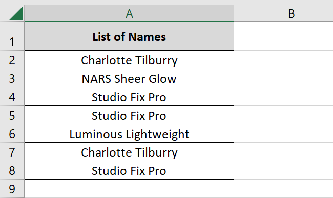
We need to remove the duplicate values from this list.
Here are different methods that can help you do this✂
Advanced Filter
To remove duplicates values from your data using the advanced filters:
- Select the data that needs to be filtered.
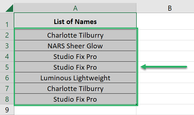
- Go to the Data Tab > Advanced Filters.

This opens up the Advanced Filter dialog box as follows 👀

The list range is already selected (that’s because we selected the data to be filtered before launching the advanced filter) 👌
Pro Tip!
Under the box Action:
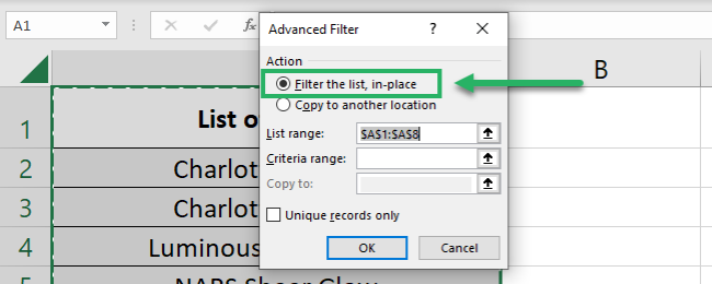
- Select Filter the list, in place if you want the original dataset to be de-duped.
- Select copy to another location if you don’t want to disturb the original data. This way Excel will ask you for a location (a cell range basically) where you want to create a copy of the source data. Duplicates will then be deleted from this copied set of data and your original data will remain the same.
- Check the option for Unique Records only. This tells Excel to delete any dupes from the dataset.
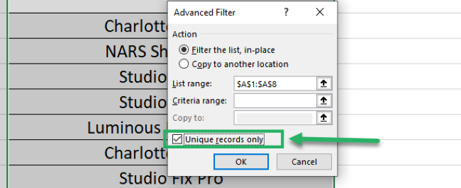
- Click Okay.
Here comes the data which no longer has duplicates 🤩
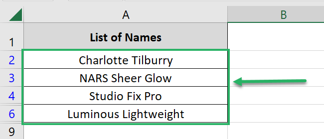
Note that we had selected the option to Filter in place so our original dataset has changed.
Remove Duplicates
Do you know Excel has an in-built feature for removing duplicates? We will explore that now 🔎
So with the same list of names, here we go:
- Select the column header for the column that contains the duplicate values (List of Names in our example).
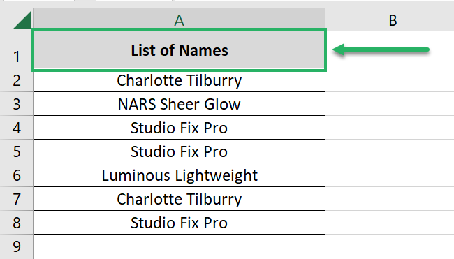
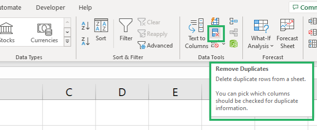
- Go to the Data Tab > Remove Duplicates.
- Select the column from where the duplicates are to be removed. Note that it is already selected in our case.
- Check the box for “My data has headers” as highlighted below.
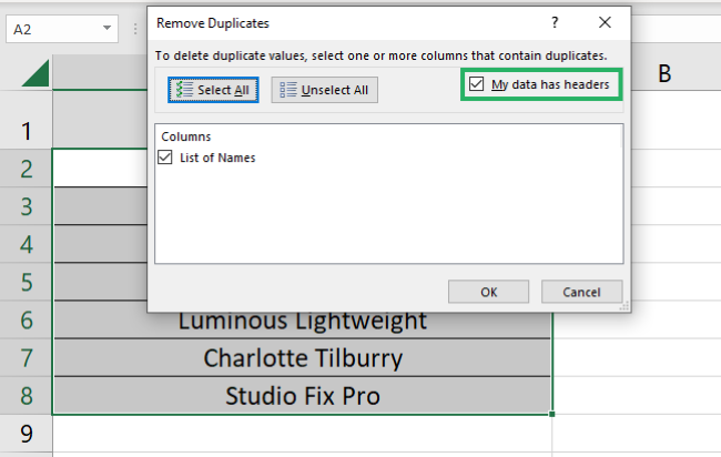
- Click Okay.
Excel brings you a dialog box that tells how many duplicate values have been found and removed. And how many unique values are retained. This way you can remove duplicates from each column of your dataset 🚀

Here is the deduped list. Excel has found and removed all instances of duplication 💪
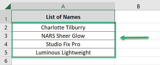
UNIQUE function
Another way how you can extract unique (or other than duplicate values) from a dataset is by using the UNIQUE function.
The UNIQUE function extracts a list of unique values from a given set of values 📝
Must know that the UNIQUE function is a dynamic array function. It returns an array of unique values 📌
And as it is a dynamic array function, it is only available in the dynamic versions of Excel. Starting from Excel 2021 to Microsoft 365 only. The older (non-dynamic versions) of Excel do not support dynamic array functions.
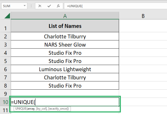
So to extract a list of unique names from our dataset:
- Begin writing the UNIQUE function as follows ✍
= UNIQUE
- Specify the range that needs to be filtered.
= UNIQUE (A2:A8)
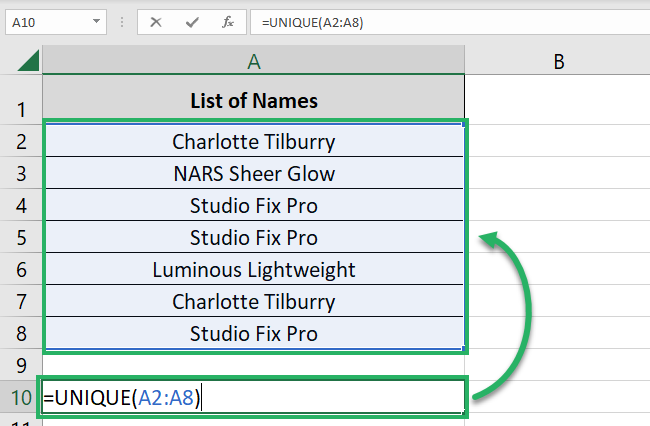
We want to remove dupes from the list of names i.e. Cell A2 to Cell A8. So we are creating a reference to these cells.
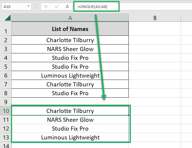
- Hit Enter, and there are your filtered values.
Pro Tip!
Instead of an array of unique values, did the UNIQUE function return the #SPILL error 🥴
That’s because your spill range is not empty (some cells might already have values). The spill range is the cell range (to the bottom or right of the active cell) where the UNIQUE function will populate the array of unique values.
How to find duplicates in excel
You’d enjoy the process of finding duplicates in Excel. Make sure you’re there with us till the end of it 🚴♀️
Continuing with the same list of names from our previous example.

This time we only need to find out the duplicate values from this list, so here we go.
- Select the data (from where you want to find the duplicates).

- Go to the Home Tab > Conditional Formatting.

- From the drop-down menu that appears, select Highlight Cell Rules > Duplicate values 🎨
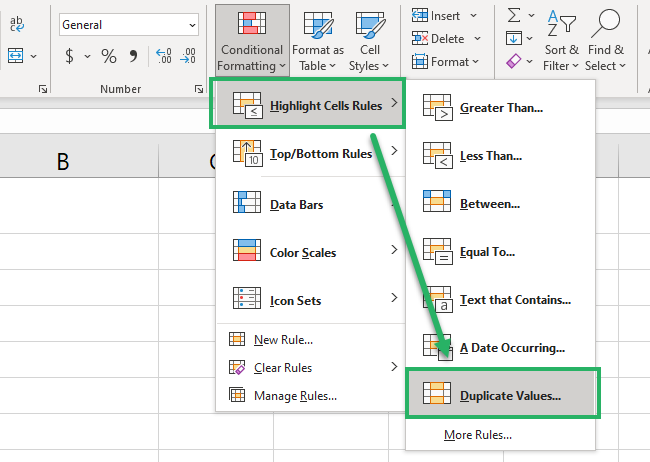
This way the conditional formatting tool of Excel will highlight duplicates from the selected dataset.
Like in the image below.
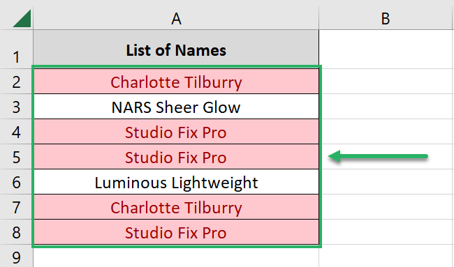
We have all the duplicate data highlighted from our dataset above.
However, all the values are still mixed. Do you want to separate the duplicate values?
Do it through the steps below 👇
- Select the header for the subject column (List of Names in our example).
- Go to the Data tab > Filter.

Once the filters are applied, you’d see the filter icon (drop-down menu icon) inside the selected column header.
- Click on that drop-down menu icon 🔽
- From the context menu that opens up, select Sort by Color > Red.
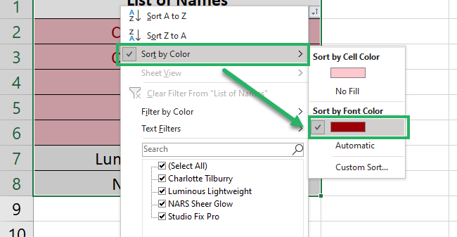
And we have the highlighted values (duplicate values) filtered only.
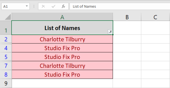
You now may choose to cut/paste them, delete them or treat them in any way you like 🙈
That’s it – Now what?
The above article is a complete guide on how to find and remove duplicates in Excel. Like reading it?
If you did, you’d be amazed to know how versatile Microsoft Excel is. And the best part of Excel is that it has a huge (and that’s an emphasized huge) library of functions 📚
Each function of Excel is super smart and useful when used the right way. To master Excel functions, you must have a good grip on some core functions of Excel.
These include the VLOOKUP, SUMIF, and IF functions. To learn them, enroll in my 30-minute free email course now. It covers these (and many more) Excel functions, features, and tools.
Other resources
Want to learn more about conditional formatting in Excel? It will help you in many ways. Click here to read our blog on it.
