How to Cut Off Text in Excel (Keep Text in Cell)
When working with large data sets, you might often come across text that exceeds the boundaries of the cell and trespasses into those adjacent to it.
Truncating text within a cell while keeping the content intact is often necessary to keep your Excel sheet clean and organized ✅
Managing text overflow in your spreadsheet is important if you want your data to be presentable, appealing and easy to navigate.
In this tutorial, we will see different ways you can use to cut off text in Excel – from wrapping text to using text boxes. Download our sample workbook here to practice along the guide 🔽
Using wrap text
One of the most common ways to cut off text in Excel is to use the wrap text feature. It fits the entire piece of text in a cell. Let’s see how to use it.
We will use the following sample data.
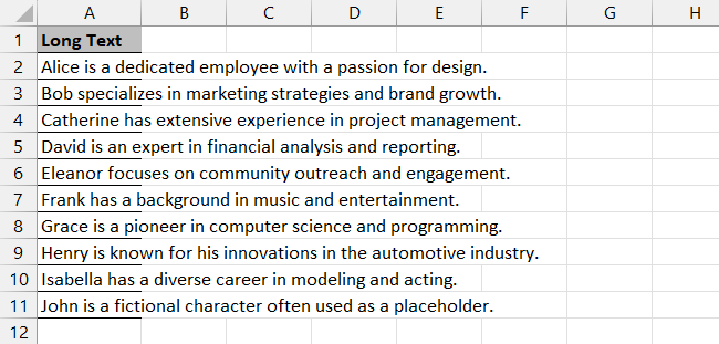
To do that,
Step 1) Select the cell you want to cut off text from.
Step 2) Go to the Home tab and select Wrap text from the Alignment section.

The text in the selected cell will be wrapped and will look something like this:
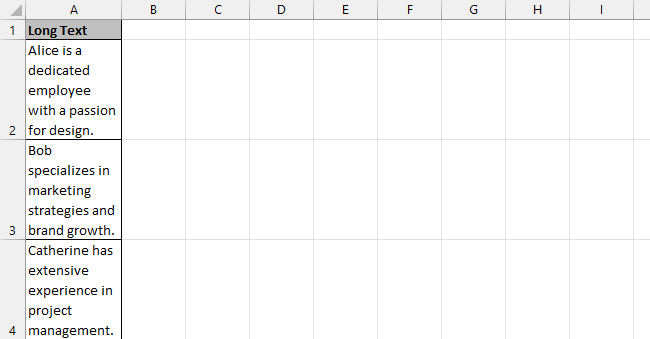
If this was how you wanted your cell to look like, you’re done here. But if you don’t want it to be this tall, we’re going to have to make some changes.
On your Home tab, click on the Format option from the Cells section and select Row Height or press Alt + H + O + H.
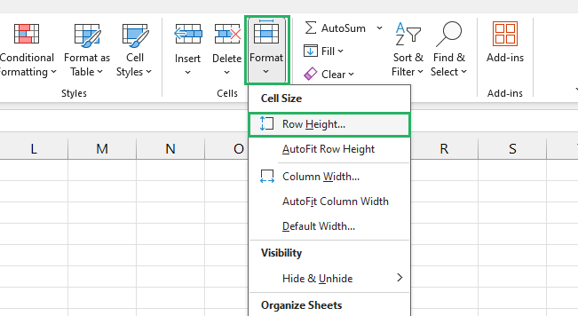
Step 3) Doing this will bring forth the Row height dialogue box.
Step 4) Set the height to 15 pts which is the default height for a row.
Step 5) Press Ok.

This will hide all the lines of text after the first one and your cell will look something like this:
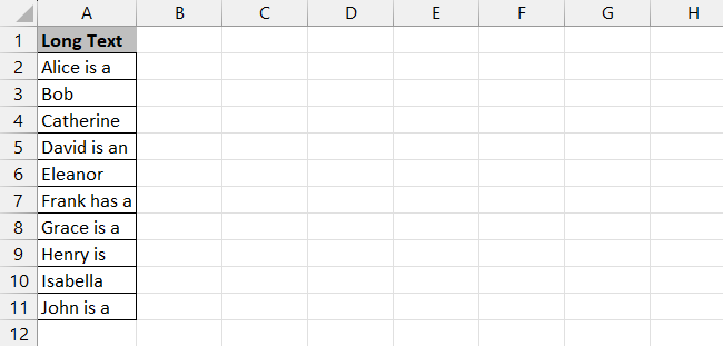
Cool, no? 😀
Using horizontal fill
Another method you can use to stop cells from spilling text over to the adjacent cells is to fill them horizontally. It truncates the text so that it only stays in the current cell.
We will use the same sample data as earlier.
To do that,
Step 1) Select the cells containing the text you want to truncate.
Step 2) Go to the Home tab and click on the Dialog Launcher at the bottom right corner of the Alignment section or press Alt + H + F + A.

Step 3) The Format Cells dialog box will appear.
Step 4) Go to the Alignment tab on the dialogue box.
Step 5) Click on the box under Horizontal and select Fill from the dropdown list.
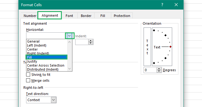
Step 6) Click Ok.
And it’s done! 🧐
The cell will be cut off at its boundaries to look something like:
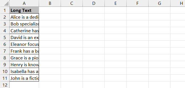
The Fill feature works perfectly if all cells extend to the other column. However, if even any one cell is shorter and doesn’t exceed the boundary of the cell, it will repeat that piece of text multiple times to fill that cell. This means a “Long-text!” string may be written as “Long-text!Long-text!”
Using shrink-to-fit
We just saw you can resize the cell to fit the length of your content but what if I tell you Excel lets you resize your content to fit the cell too? Let’s see how to do that below 🔽
We have the same sample data as earlier.
To shrink text to fit,
Step 1) Select the cell you want to shrink text in.
Step 2) Go to the Home tab and click on the Dialog Launcher at the bottom right corner of the Alignment section or press CTRL + 1.

Step 3) The Format Cells dialog box will appear.
Step 4) Go to the Alignment tab on the dialogue box.
Step 5) Select Shrink to fit from Text Control.
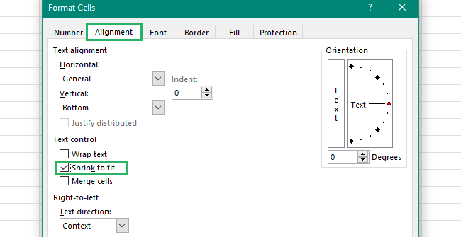
The text in the cell will be shrunk to fit the size as :
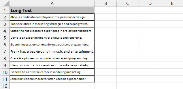
However, as evident, shrinking the text in the cell makes legibility a critical issue. For this reason, it is suggested to only use the shrink-to-fit option when the text is only a couple of characters longer than the cell size. This removes room for complications.
Using Excel formulas
If your dataset is rather symmetrical, you can use Excel formulas to work with all of them in one go. We will use two functions, LEFT and RIGHT.
The purpose of these functions is to retain a certain number of characters from the left or right and remove the remaining. Let’s see how to do that below.
LEFT Function
The left function removes the given number of characters from the left side of the cell. It is one of the most commonly used functions when it comes to cutting off text in Excel. Let’s see how to do it.
Its syntax is given as follows:
where,
Text refers to the string you want to truncate
Num_chars refers to the number of characters you want to retain – this is an optional argument
We will use the following sample data set.
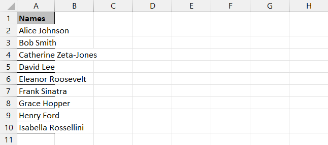
To use the left function,
Step 1) Select cell B2.
Step 2) Type in the following formula:
Step 3) Press Enter.
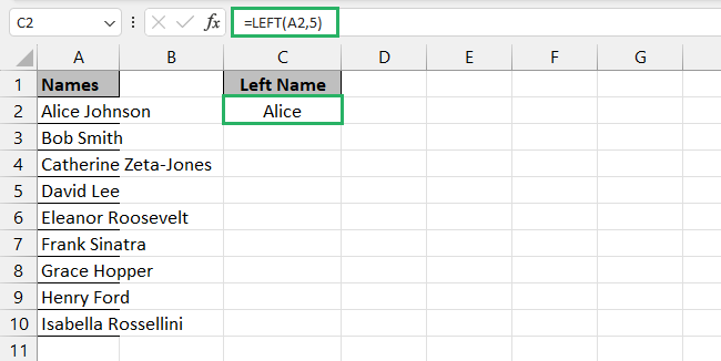
The formula will retain the first six characters of the text in cell A2 and remove others.🚩
You can copy the formula down to the remaining cells if you want to remove the same number of characters from each cell.
However, if each cell contains a different number of characters to be truncated, this formula can be a little difficult to handle.
RIGHT Function
The RIGHT function works similarly to the LEFT function. Let’s see how.
Its syntax is given as follows:
where,
Text refers to the string you want to truncate
Num_chars refers to the number of characters you want to retain – this is an optional argument
We will use the same sample data set as earlier.
To use the right function,
Step 1) Select cell B2.
Step 2) Type in the following formula:
Step 3) Press Enter.
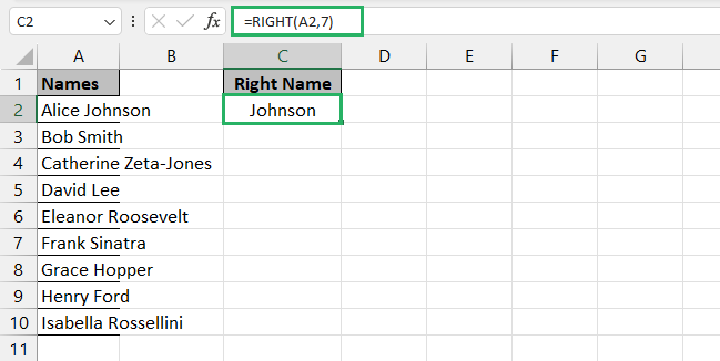
The formula will remove all characters from the cell except for the last four from the right.
Isn’t this cool? Try now! 🤯
Adjusting column width
One of the fastest ways to cut off text in a cell in Excel is to adjust the column width. Note that this method resizes the entire column you are working on and not just a single cell.
You can adjust it either automatically or manually. Let’s see both the methods below. We will use the same sample data set in both cases.
Adjust Column Width
In this case, you manually adjust a column width by entering the desired width points.
To do that,
Step 1) Select the cells whose column width you want to adjust.
Step 2) Go to the Home tab and select Format from the Cells section or press Alt + H + O + W.

Step 3) This will launch a small Column Width dialogue box.
Step 4) Enter the size of your column according to the length of your text – we put it to 54.
Step 5) Press Ok.

The column will be resized to the set width as:
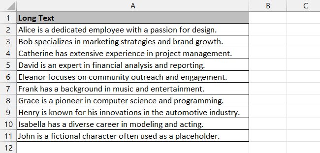
Easy, right? 🤓
Autofit Column Width
This method requires an even lesser number of steps than the above one and is certainly a favorite – especially when you use its shortcut key 😎
To autofit column width,
Step 1) Select the cells whose column width you want to adjust.
Step 2) Go to the Home tab and select Format from the Cells section or press Alt + H + O + W.

And it’s done! The column width will be resized according to the length of the text in the cell.

Note that when you autofit column width, it automatically sets the width of all selected cells according to the longest string in each cell. This might make your data look a little out of order if you want a rather symmetric look on the data set.
Using text box for custom display
Another hack to cut off text in your worksheet is to use a text box that lets you customize how you want to display your text. Let’s see how to do it below.
We will use the same sample data as earlier.
To do that,
Step 1) Go to the Insert tab and click on the Text box from the Text section.

Step 2) Once it’s activated, draw a text box on the screen.
Step 3) Select the cell containing the text and press CTRL + C.
Step 4) Place your cursor in the text box and press CTRL + V to paste the cell contents.

Your text is now in the text box. You can resize the box as you want to fit the text.
How fun is that? 😃
Conclusion
In this guide, we saw different ways of cutting off text in Microsoft Excel. We saw how to wrap text in a cell when it extends outside the border to use horizontal fill.
We also saw how to shrink the contents of a cell to fit it and adjust the column’s width. To take things to an advanced level, we also used Excel formulas and text boxes for custom lengths of text.
To learn more about Excel’s cells, columns and text boxes, give the below articles a read.
How to Adjust Column Width in Excel: Step-by-Step (2024)
How to Apply an Excel Formula to Multiple Cells
How to Insert a Text Box in Excel: Step-by-Step (2024)
We hope you enjoy reading this as much as we did crafting it! 🤗
