How to Apply an Excel Formula to Multiple Cells
This guide is going to be about different methods of applying an Excel formula across a magnitude of cells to enhance your productivity and work efficiency.
The core purpose of modern-day spread-sheeting is to minimize tedious tasks and streamline workflows by focusing on efficiency. This can be very well achieved if you write a formula once, and Excel automatically updates and populates it for all the desired cells 😎
To learn more about how to do this in Microsoft Excel, let’s dive into this guide. And do not forget to grab your free practice workbook for this tutorial here.
Using the Fill Handle
The most common method we all know of applying a formula to a heap of cells in Excel is to drag it all the way along.
To drag formulas in literally all four directions, we use the Fill Handle. See here 👀
We have two sets of numbers that are to be summed up.
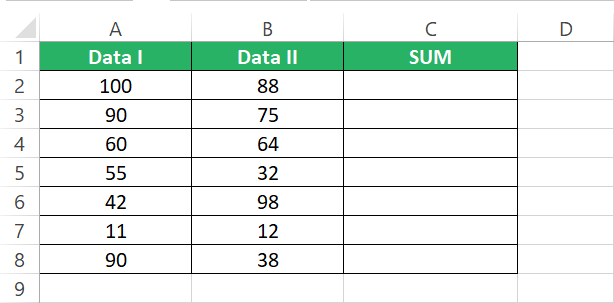
Step 1) Write a simple formula to sum the numbers in the second row.
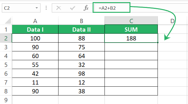
Step 2) Click on the cell containing the formula and hover to the right bottom of the cell to see the Fill Handle (a small black plus icon).
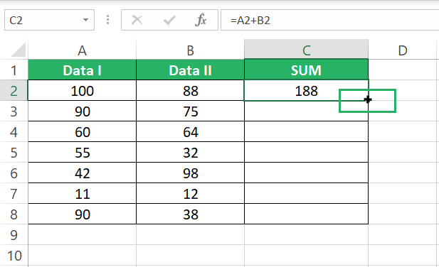
Step 3) Once you see it, drag it down to the remaining cells.’

Excel will apply the same formula by updating the cell references for all the remaining cells.
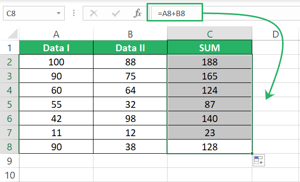
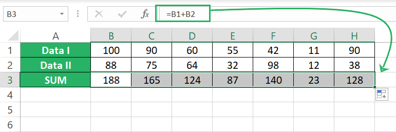
The best part about the Fill handle is that you can use it in literally any direction.
For example, if a formula sits at the end of a column.
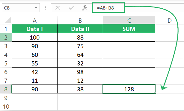
You can drag it all the way up.
Or you can drag it to the right.
Or to the left.
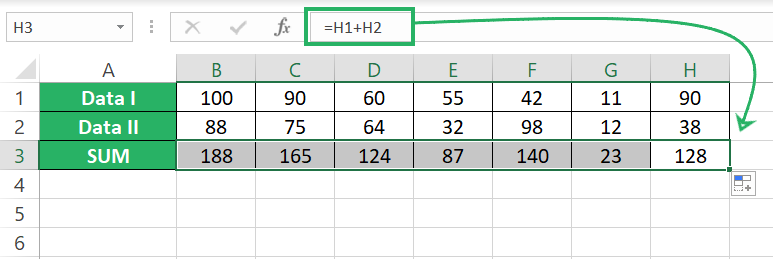
The Fill handle just doesn’t mind. Cool, isn’t it?
Absolute Cell References
While you play around with formulas applying them to multiple cells, you must know how Excel updates the cell references when a formula is applied to a different cell.
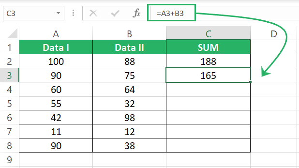
For example, I wrote a simple formula to add cells A2 and B2 in the example above.

As I drag it a row down, Excel will automatically update the formula to take the cell references a row down i.e. A3 and B3.
While I can never explain enough how big of a lifesaver this feature is, in some cases, you might want one or more cell references to remain the same and not update as the formula changes cells.
For instance, in this case, I need to see what amount is saved on each item when I apply a 10% discount to it. So, I will multiply 10% (in Cell B7) by all the items individually 🛒
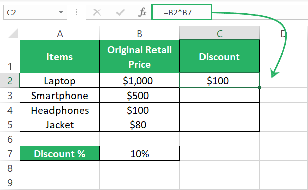
Now as I drag the formula down, I do want the cell reference for prices to update but not the cell reference for B7 (that contains the discount rate).
To help this situation, we use absolute cell references.
Within the formula, I will click on cell reference B7 and press down the F4 key to convert this reference to an absolute reference (see the dollar signs that come apprehended to it).
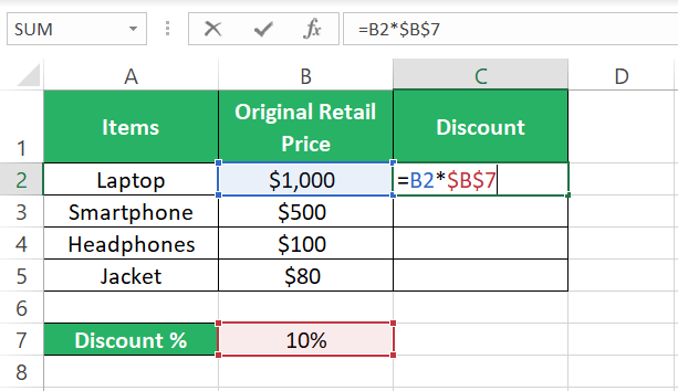
Now when you drag this formula down (or in literally any direction), the Cell reference B7 won’t change.
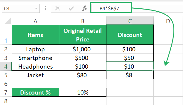
You can convert the whole cell reference into an absolute one like $B$7 or only the column letter reference ($B7) or row number reference (B$7) into an absolute one.
Using Ctrl + D & Ctrl + R
If you are a pro typist who just doesn’t want to slow down their pace by reaching out for a cursor again and again, these keyboard shortcuts are for you.
To drag a formula down, you do not necessarily have to use the Fill handle, instead, you can use the Control key + D shortcut 💻
Step 1) Select the cell containing the formula.
Step 2) Press down the Shift key and down arrow up until you select all the cells where you want the formula applied.

Like this:
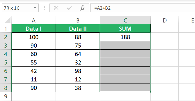
Step 3) Press the Control key + D.

Excel will copy the formula down across all the cells.
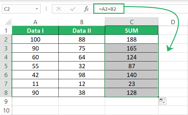
Similarly, to drag it towards the right.
Step 1) Select the cell containing the formula.
Step 2) Press down the Shift key and right arrow up until you select all the cells where you want the formula applied.

Step 3) Press the Control key + R.
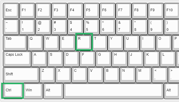
Excel will copy the formula towards the right across all the cells.

It’s all about the keys – no need to use the cursor whatsoever 🖱
Using Ctrl + Enter
Control + Enter is a magic trick to take formulas across a cell range in a jiffy.
For instance, if I want to find the sum of all the numbers from the columns Data-I and Data-II in one go, here’s what I will do:
Step 1) Select the first cell of the range (i.e., C2).
Step 2) Press down the shift key + the down arrow until you’ve selected all the cells and where the formula is to be applied.
Step 3) Press the ‘equal sign’ on your keyboard.
This will activate the first cell of the selected range.
Step 4) Type in the following formula.
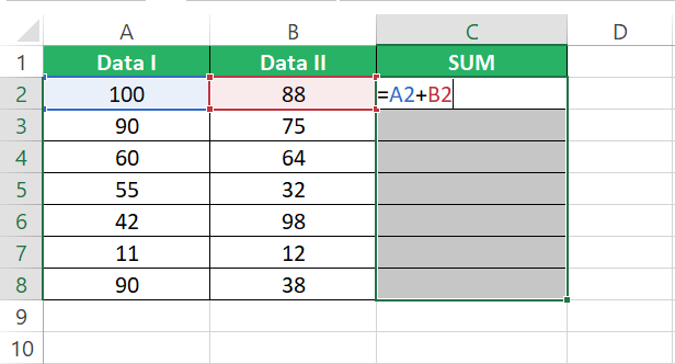
Step 5) This is the most important step – unlike other formulas, don’t just press the ‘Enter’ key but the Control key + Enter key in combination.

The formula will be applied across all the selected cells, just like that.
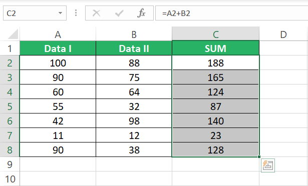
Jaw dropped? There’s more to come 😄
Using Dynamic Array Formulas
This section is only going to work around for Microsoft Office 365 users.
Dynamic array formulas do not work for the previous versions of Excel.
Step 1) To convert a simple formula into a dynamic array formula, write it as:
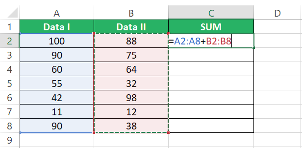
Step 2) Press Enter.
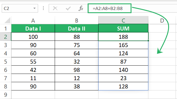
The result for the whole column is populated at once. However, it is an array. Within an array, you cannot edit/delete a single cell ❌
As you attempt to do so, Excel will give the following #SPILL! Error.
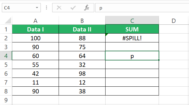
Whatever is done, has to be done about the complete array.
For example, if you want to delete this array, you must select the whole array (or the cell that contains the array formula) and then press Delete. Attempting to delete any single cell of the array will not help.
Similarly, to make any edits to the formula, you must activate the cell where the array formula is originally written i.e., Cell C2.
Using Copy / Paste
Unpopular but yes, you can also apply an Excel formula to multiple cells by copying and pasting it.
See here.
Step 1) Copy the formula in Cell C2 by pressing the Control key + C.
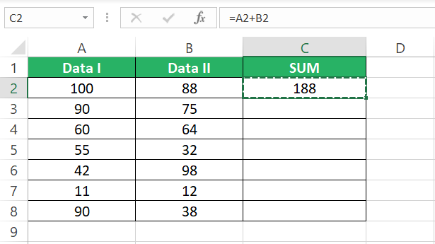
Step 2) Select all the cells where you want the formula pasted.
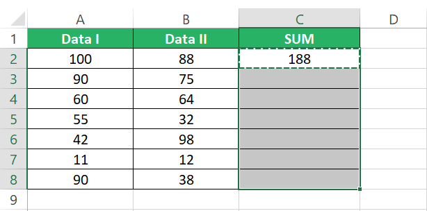
Step 3) Press the Control key + V to paste it.
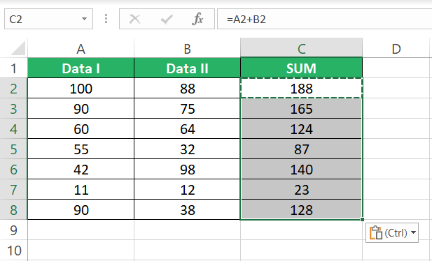
Excel will paste the formula and update the cell references for you 🏸
Using Excel Tables
Excel tables are an excellent way to synchronize your data. Plus point: they are simple to create and easy to use.
See here. Here’s our data set.
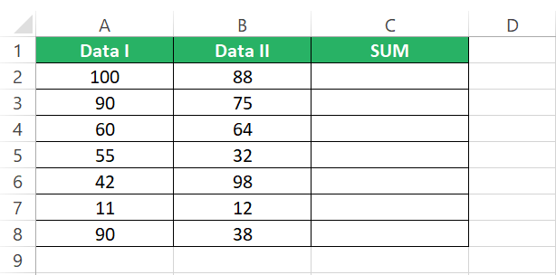
Step 1) Select it all.
Step 2) Press the Control key + T to convert it into a table.
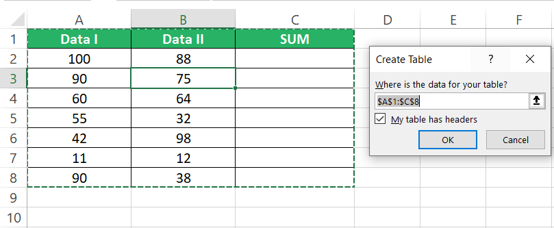
Step 3) Once converted, write the formula in any cell of the table and hit Enter 🏓
Excel will automatically stretch it across the whole column/row for the adjacent cells.
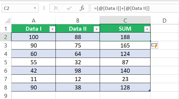
Once you’ve got the results, you may want to convert the table back into a simple range of cells.
Step 4) For that, just select any cell of the table.
Step 5) Go to the Table Design tab > Tools > Convert to Range.

Excel will convert the table back into a simple range.
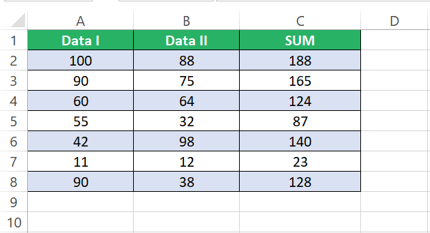
Alternatively, if you are more of a keyboard person, you can also use sticky keys to convert a table back into a simple cell range.
Press the Alt key > JT > G. Sticky keys are always to be pressed in sequential order (i.e., one after another and not together).
Conclusion
This guide brings together a great deal of techniques that you can use to apply a formula productively and efficiently to multiple cells in Excel.
However, this is just the tip of the iceberg when it comes to Excel’s capabilities.
To explore other cool tools and features of Excel that you can leverage to take your Excel game up and beyond, go ahead and read my following Excel tutorials.
