How to Insert A Dollar Sign ($) In An Excel Formula

The dollar sign in Excel is a simple but very powerful feature of this spreadsheet software. It gives you control over how you want to manage your cell references and formulas ➗

By placing the dollar sign at different places in cells, you can lock the cells partially and completely as you like as you drag the formula across a range of cells in your worksheet 📗

In this tutorial, we will see what a dollar sign in Excel is, and what it represents and you can use it in your Excel spreadsheet. Download our sample workbook below to practice along the guide.

Table of Contents

What is cell reference in Excel?

Cell reference in Excel simply refers to the address of a cell. In a formula, it is the cell containing the value that you want to use in the formula 💻

For example, in =A1*3, cell A1 is the reference which contains the value you want to multiply 3 with as here:

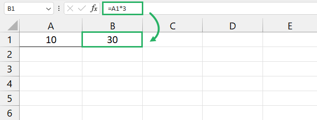
The cell reference type doesn’t matter much in this formula as it is restricted to a single cell. But if you want to copy this formula down a couple of rows, you would need to use the appropriate type.

Types of cell references in Excel

There are three types of cell references in Excel, relative, absolute and mixed reference. Let’s see what each of these are and which might be the best option for you below 😀

Relative cell reference

A cell with relative relative doesn’t have the dollar sign in its address. Its reference becomes important as you use it in a formula and then use that formula somewhere else or copy it.

The cell reference in that formula will change based on the relative position of rows and columns. This means if you were to write =A2*10 in cell B2 where A2’s value is 10, you would get a 100.

But if you were to copy the same formula to cell C2, the formula would return a 1000. That’s because it now references cell B2 instead of cell A1 🤔

That’s how cell references work. All cell references in Excel are relative by default and this is the feature we use when we want our formula to return different results based on a column of values.

Let’s see an example of a relative cell reference below.

Say, we have the following sample data where we check if the value in column A is greater than 20. If it is, the formula will return a “Pass” otherwise an empty string.

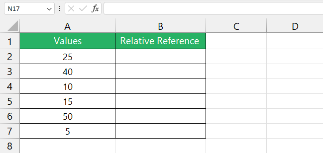
To do that,

Step 1) Select cell B2.

Step 2) Type in the following formula:

Step 3) Press Enter.

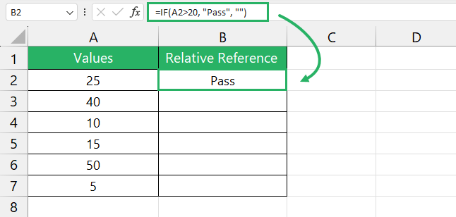
The formula will return our expected. Here comes the important part, we want to get the same result for the remaining values using our relative references.

To do that, simply double-click the Fill Handle at the bottom right corner of the cell ➕

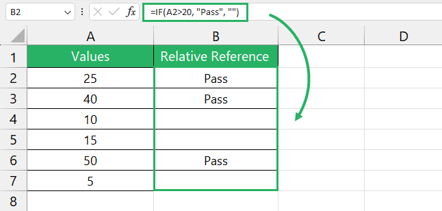
And it’s done. Using relative reference, we copied the formula down the remaining cells easily. This is one of the most common and important uses of relative reference 😀

Absolute cell reference

An absolute cell reference is the complete opposite of a relative cell reference. An absolute cell reference in a cell will not change no matter where you copy the cell or how you move it.

An absolute cell reference is written like $B$1 where the dollar shows that both its rows are coordinated and column coordinates are locked 🔒

Let’s see an example of absolute reference below.

Say, we have the following sample data where we want to calculate tax on each employee’s salary. The tax percentage is 10%, 20% and 30% but I only want to use 10% in my calculations.

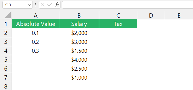
To make sure the cell address remains the same, we will use absolute cell reference step by step below.

Step 1) Select cell C2.

Step 2) Type in the following formula

Step 3) Press Enter.

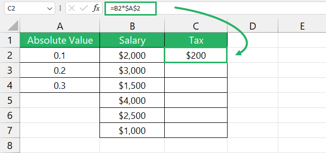
Copy the formula down using the Fill Handle 🧾

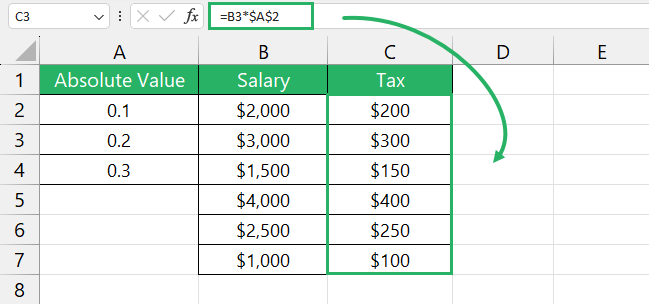
Note that the absolute value for tax did not change any cell. That is because we used an absolute cell reference that remains the same no matter how you use it.

How cool is that? 😉

Mixed cell reference

A mixed cell reference is one where one of the two things is fixed – either the row number or the column name, i.e., B$1 or $B1. It only takes a single dollar sign 💲

Absolute row reference and relative column reference or $B1 means that as you copy a formula sideways this this cell address, the column name will change to $C1, $D1 and so on but the row number will not change.

Absolute column reference and relative row reference or B$1 means that as you copy a formula down some cells, the column name will remain the same but the row number will change as C$1, D$1, similar to what we saw in relative reference.

Let’s see an example related to mixed cell reference below.

Say, we have the following sample data in your Excel sheet that contains a list of weekly targets and taxes for different months. We want to find the product of target and tax for each month.

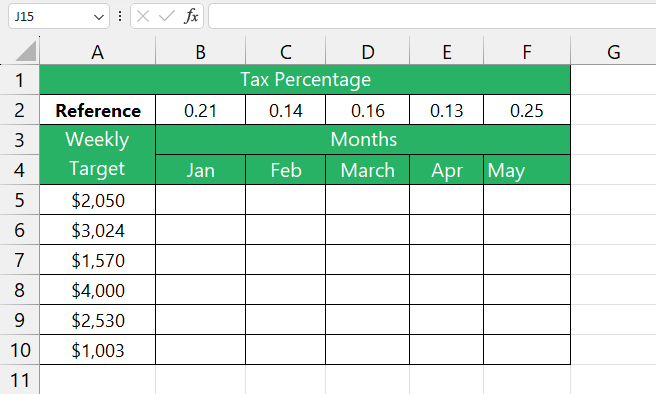
To do that,

Step 1) Select cell F3.

Step 2) Type in the following formula:

Step 3) Press Enter.

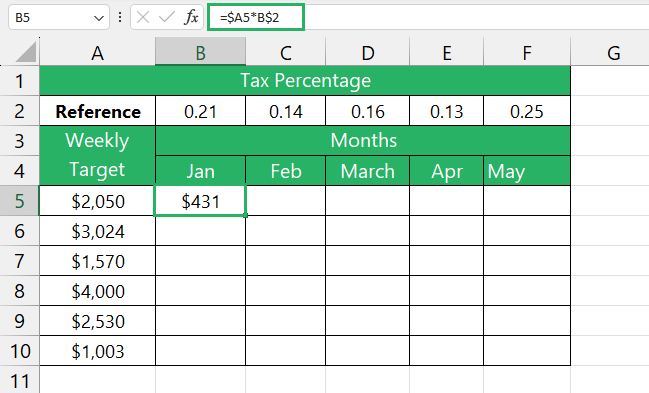
Now copy this formula to the right of your range to see how relative column reference works.

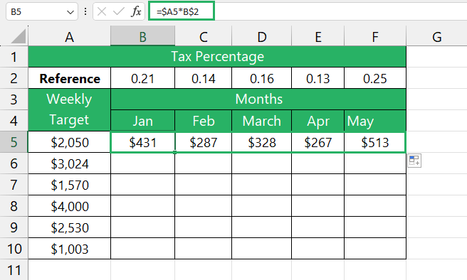
Now copy the formula in cell B5 down to see the relative row reference in action.

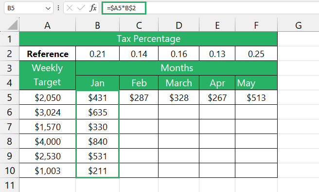
Do the same for the remaining columns:

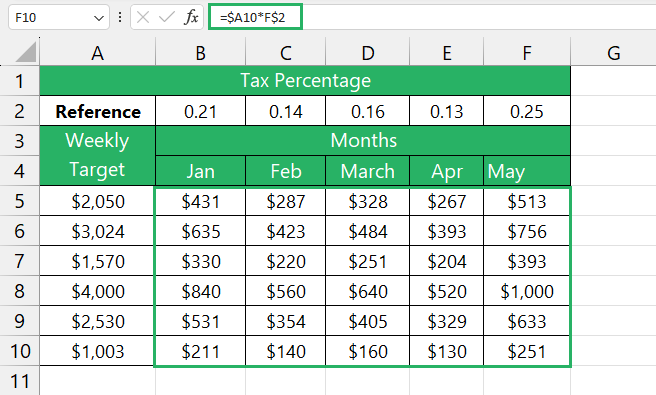
See? With such a small formula, we were able to fill in 30 cells of data. How cool is that? 😀

How to insert a dollar sign in a formula

Let’s now see how you can insert this dollar sign in an MS Excel formula. There are three ways you can use to achieve this which are as follows:

Manually

You can insert the $ sign manually at the start and end of a cell reference. Simply place your cursor before the column name like before A1, and insert the dollar sign as $A1 💲

So the same for column names to get something like A$1 and $A$1. Adding dollar sign manually is a bit of a hassle and can seem very unprofessional but sometimes it might be the fastest option for beginners mastering Excel.

Using find and replace

You can also use find and replace to insert a dollar sign in a formula. Simply look for the cell reference containing the base value and replace it with the desired reference as:

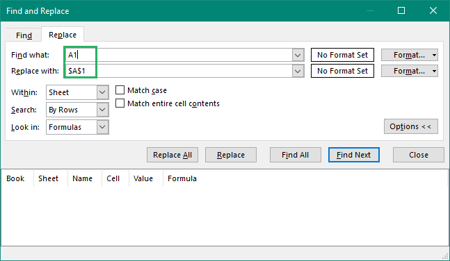
This method is easier than manually inserting the dollar symbol but if you have different column letters for all references in your formula, it can get a bit tiring 🥱

Using F4 shortcut key

The quickest and most usable method is to use the F4 shortcut key. It is a keyboard shortcut that toggles between absolute, relative and mixed cell references.

You can choose whichever you like and even if you miss it the first time, you can toggle again to go back to it 🔁

Simply place your cursor next to the cell address whose reference you want to change and press the f4 key. It will change the reference to:

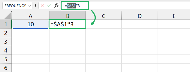
Pretty cool, no? Try it now! 😎

Conclusion

In this tutorial, we saw different methods of how to insert the dollar sign in a formula in Microsoft Excel. We saw what a cell reference was, its types and how it works.

To learn more about cell references in Excel, read the articles below 📑

Cell References in Excel: Relative, Absolute, and Mixed (2024)

How to Apply Excel Formula to Entire Column (Easy)

We hope you enjoyed reading this article as much as we did creating it 🤗