How to Apply Excel Formula to Entire Column (Easy)
Excel’s ability to apply formulas across a whole column in a single go makes it a superhero for number crunching🔢
Dragging a formula’s power down the whole column helps you save loads of time. It makes working just so much more efficient and accurate.
There are multiple ways how you can apply an Excel formula to an entire column. Read with me through the end to explore all the possible ways how you can make the best use of this game-changing feature of Excel.
Don’t forget to grab your free practice workbook for this guide here.
Double-click the Fill Handle
I have two columns of numbers in Excel, and I want to sum Number 1 and Number 2 from each row➕

After we’ve devised the formula for the first row (a simple A2+B2), we will apply it to the entire list of numbers using the fill handle by following the steps below.
Step 1) Select the cell that contains the formula.
Step 2) Hover your cursor around the lower-right corner of this cell to see a plus icon.

This plus icon is what we call the Fill Handle.
Step 3) Once you see it, place your cursor on it and double-click it.
The Fill Handle comes into action and fills the formula across all the upcoming cells.
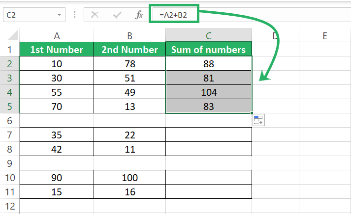
But it didn’t do so for the entire list. The automatic formula filling stops at Cell C5. Strange?
If you have an adjacent column to the column where you’re applying the formula and that column contains any blank cell, the Fill Handle will only fill formulas up to that cell.
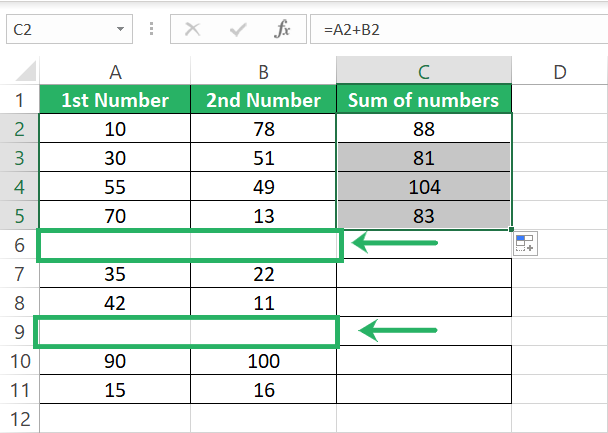
Step 4) For the remaining cells, you’d again have to write the formula in Cell C7.
Step 5) And double-click the Fill Handle again.
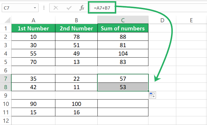
We again have another empty adjacent cell in between which is Cell B9.
Step 6) Again, write the formula for the next cell i.e., Cell C10.
Step 7) Double-click the Fill Handle around Cell C10 to apply the formula to the cells that come next.
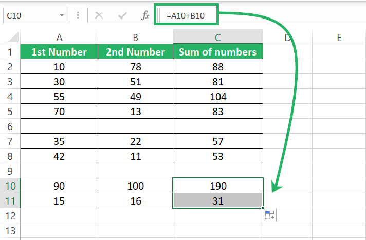
This method works best when you have no space instances in your data👀
Drag down the Fill Handle
The main problem with double-clicking the fill handle is that it stops at the point where there are any empty cells in the adjacent column.
However, you can help this problem by dragging down the fill handle yourself.
Step 1) Start by writing the formula for the first cell.
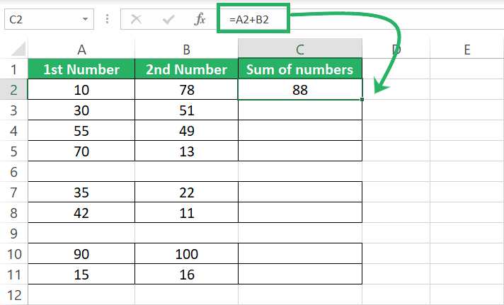
Step 2) Select the cell that contains the formula.
Step 3) Hover your cursor around the lower-right corner of this cell to see the Fill Handle.
Step 4) Once you see it, place your cursor on it and drag it down to the cell where you want the formula applied.
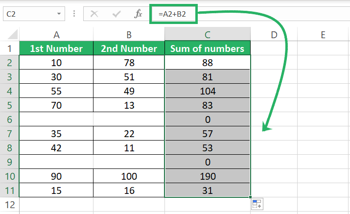
As you are manually dragging it down, even if there are any empty adjacent cells in between, Excel will still apply the formula for those🚀
Use the Fill Down button
Excel also has an in-built button to help the application of a formula across an entire column. We call it the Fill Down Button and it’s located in the ribbon.
Step 1) Write up your formula for the first cell.
Step 2) Select the range of cells to which you want the formula applied.
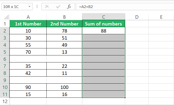
Step 3) Go to the Home Tab > Editing Group > Fill.
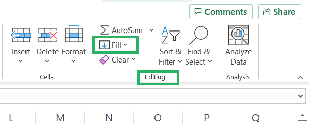
Step 4) Click on the Fill button to launch the drop-down menu of options > select “Fill Down”.
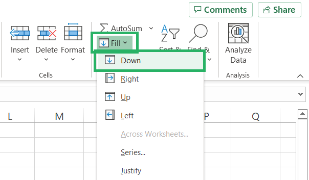
That’s it – Excel copies the formula down all the selected cells 🏍
Can also add it to the Quick Access Toolbar
If you have a lot of work to do with applying formulas across the column in Excel, you can add the Fill Down button to your Quick Access Toolbar for easy access.
The Quick Access Toolbar appears on the top of your Excel workbook.

Fill Down the button to your Quick Access Toolbar:
Step 1) Click on this small dash + arrow icon on the Quick Access Toolbar.

Step 2) From the menu of options, select More Commands.

Takes you to the Excel Options windowpane.
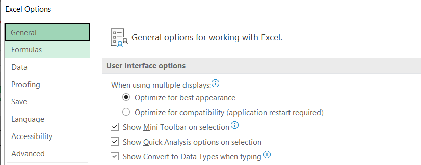
Can’t find the small dash + arrow icon? You can launch Excel Options by going to the File Tab > Options.
Step 3) From the Excel options windowpane, select Quick Access Toolbar.
Step 4) From the Option on top to Choose Commands from, select a Home tab (since the Fill Down button appears in the Editing Group on the Home tab).
Step 5) Search for the Down Fill button.
Step 6) Click on Add.
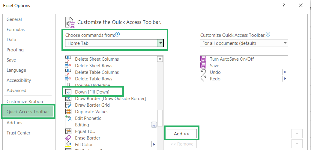
Step 7) Once added, it will appear in the box on the right.
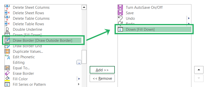
Step 8) Click Okay.
The Fill Down button is now added to your Quick Access Toolbar as an icon.
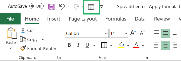
Now you can quickly click on this button to apply a formula across a selected range of cells 🤩
Copy / Paste the formula
You can also copy a formula and paste it into as many cells as you want.
This works the same as dragging a formula across multiple cells as when you copy/paste a formula, Excel automatically updates the cell references for the pasted formulas.
Step 1) Select and copy (Control + C key) the formula from Cell C2.
Step 2) Select the range of cells where you want the formula applied (Cell C3 to C11).
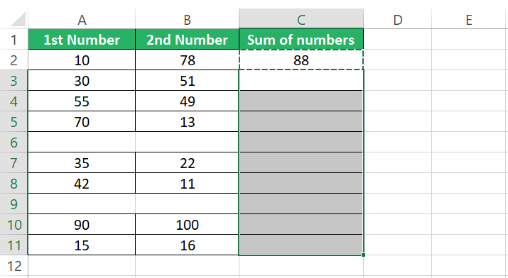
Step 3) Press the Control key + V to paste the formula.
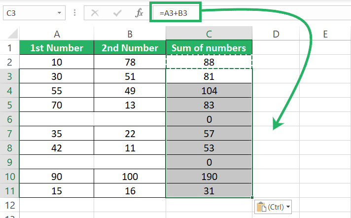
You’d see the formula pasted across the selected cells just like we do it by other methods.
Hold down Ctrl +D (Shortcut keys)
You can also apply a formula to an entire column without having to use your mouse at all. But by using keyboard shortcuts ⌨
Step 1) Write up your formula for the first cell.
Step 2) Select the range of cells to which you want the formula applied.

Step 3) Press the Control key + D.
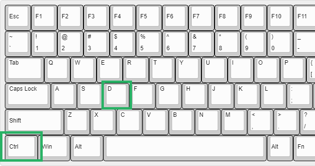
This is the shortcut key for Fill Down and it applies the formula down to all the selected cells.
Use an Array Formula
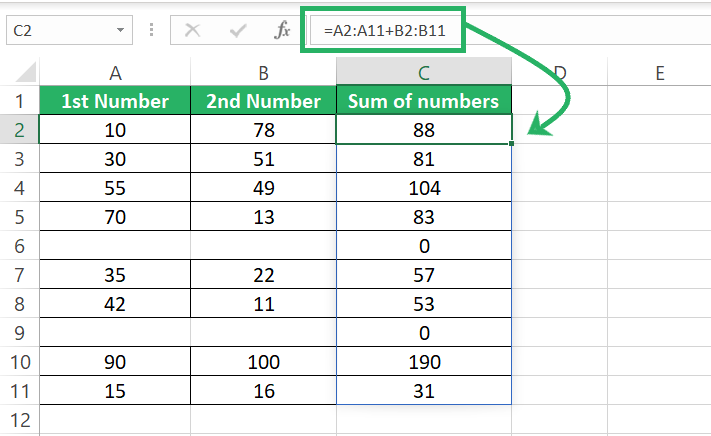
How about you write a single formula, and it automatically covers an entire column?
Yes, this is possible with the array formulas of Excel.
Step 1) To find the sum of all numbers within Column A and Column B, we can write an array formula as:
Step 2) Press Ctrl + Enter to have the array formula applied across the entire specified cell range.
Look out for these!
We have seen all the possible methods that you can use in Excel to take your formula down an entire column. Look out for the following important aspects of formula auto-filling in Excel.
Absolute / Relative references
An absolute reference in Excel means a cell reference where both the column and row references are suffixed by a dollar sign ($). Like Cell $A$4.
This tells Excel to lock the cell reference and not to update it as the formula changes cells 🔒
All other references are relative references. Excel updates these references based on cell movement.
For example, if I want to find 15% of the values in Column A, I will write the formula as:
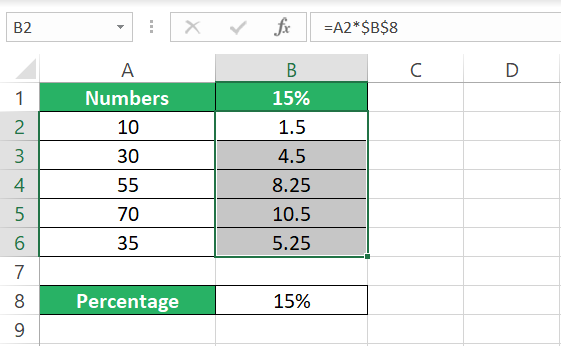
I have used an absolute cell reference for $B$8 so that it doesn’t change as I drag and drop the formula to the remaining cells.
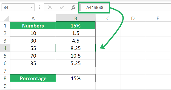
Had I used a relative reference for it, Excel would have changed it for every successive cell upon the formula being dragged leading to erroneous results.
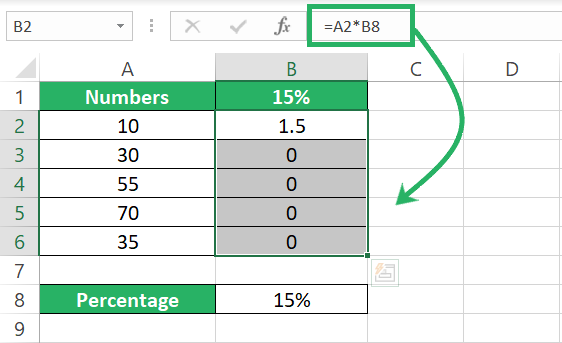
While you apply formulas across multiple cells in Excel, take care of your cell references based on the situation.
To turn a cell reference into absolute, select a cell > press the F2 key > take your cursor to that particular cell reference and > press the F4 key.
Automatic Calculation Enabled or Disabled?
To make your formulas work in the best order when taken across multiple cells, make sure to have the automatic recalculation of cells enabled in Excel.
Step 1) Double-check it by going to the Formulas tab > Calculation Group > Calculation Options.
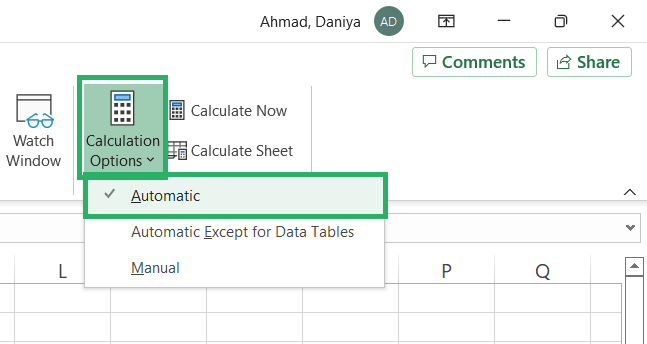
Step 2) The calculation mode must be set to automatic.
The Fill Handle doesn’t show up
If you’re hovering around a cell trying to find the Fill Handle, but it just won’t show up – you’ve some settings out of order 🤯
Most probably, the “fill handle and cell drag and drop” option is disabled. Here’s how you can enable it:
Step 1) Click on the File tab > Options.
Step 2) In the Excel Options dialog box, go to the Advanced tab from the pane on the left.
Step 3) Go to the Editing options section.
Step 4) Check the “Enable fill handle and cell drag-and-drop” option.
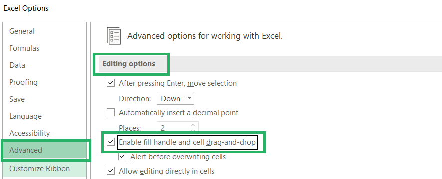
After the Fill Handle option is enabled, you should be able to see the Fill Handle again.
Formatting Copied across the cells
With all the methods discussed above (except for the array formula), whenever you apply a formula across multiple cells, the formatting of the source cells along with the formula will also apply to the destination cells.
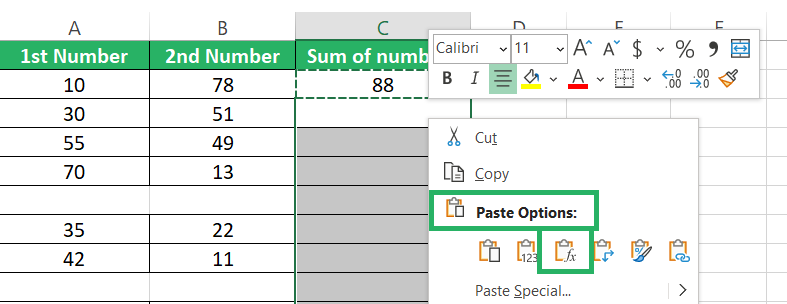
Under the copy/pasting method, this can be fixed through the “Paste only Formulas” option.
However, to fix this (copy only the formula but not the formatting) for the other methods, follow these steps:
Step 1) Once you have dragged/double-clicked the fill handle to have the formula auto-filled, you’ll see the Auto Fill Options icon here.
Step 2) Click on the small drop-down menu icon next to it.

Step 3) From the menu of options that comes then, select the option to Fill Without Formatting.
Excel will instantly remove the formatting from the cells where the formula was dragged 🧹
Conclusion
This was a comprehensive tutorial that discussed all the possible methods to effortlessly extend a formula’s power down a column in Excel.
Plus, we’ve also seen some “ifs and whens” related to formula dragging in Excel to know how to make the best use of this basic, yet very powerful tool.
This feature of Excel, though basic, makes Excel a powerhouse of efficiency. If you’re a fan of Excel’s formula drag and drop feature like me, I am sure you’d love the following tools of Excel, too.
Read out my Excel tutorials on them to learn how to use them.
