How to Use the FILTER Function in Excel + Examples
If you had to filter in Excel, what would you normally do?
Use filters, or if the filtering gets more complex, use advanced filters. Both these tools, though very useful, come with one major drawback🤔
They do not update automatically as you update the underlying dataset. But to help this out, we now have the FILTER function. It automatically updates as the data changes.
How to use it? Let’s learn that in the guide below with the help of our sample workbook you can download here.
Table of Contents
How to use the FILTER function (basic)
The FILTER function comes from the dynamic array functions’ family of Excel.
The FILTER function is only available in Microsoft 365 and Excel 2021. The older versions of Excel do not have this function.
It will not make changes to the original data. Instead, it will filter out data (based on the criteria you supply) in a separate location. Let’s test out a basic example to see how it works💡
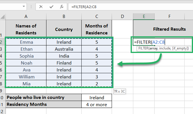
Here we have a dataset that includes a list of people, their countries, and months of residence in there.
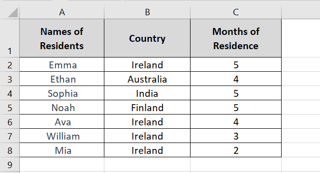
From this data, let’s filter out people who reside in Ireland only🌎
- Write the FILTER function as follows:
= FILTER
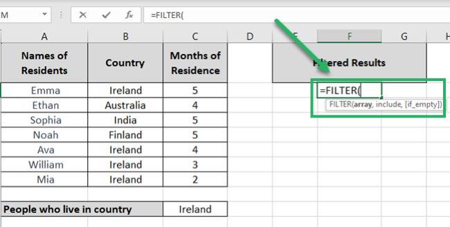
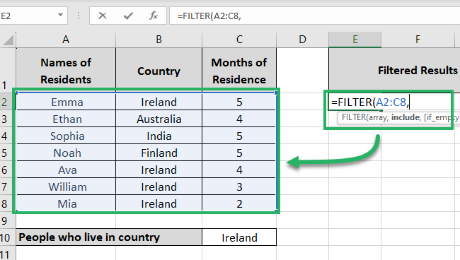
- The first argument specifies the array from where the data is to be filtered.
We will specify this range as A2:C8.
= FILTER (A2:C8,
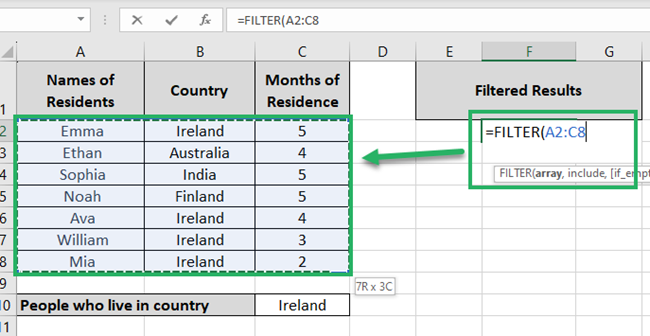
If you don’t want all the details to be filtered out. For example, if you only want the names of the people who live in Ireland filtered out (and not the country and residency months), specify the array as A2:A8 only📜
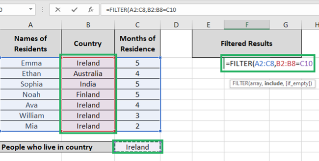
- The second argument of the FILTER function is the include argument. This is where we define the criteria.
Column B contains the country, and as we want to filter out the people who live in Ireland, so our criterion would be B2:B8=”Ireland”.
We have Ireland written in cell C10 so, we are referring to it instead of hardcoding Ireland👇
= FILTER (A2:C8, B2:B8=C10,
- The last argument is if_empty. This will be returned if the FILTER function fails to find values that fit the specified criterion.
You can leave it blank or set it to any desired value. We are setting it to “Not Found”.
= FILTER (A2:C8, B2:B8=C10, “Not Found”)
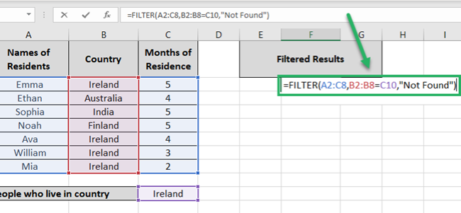
- That’s it. Hit Enter🏃♀️
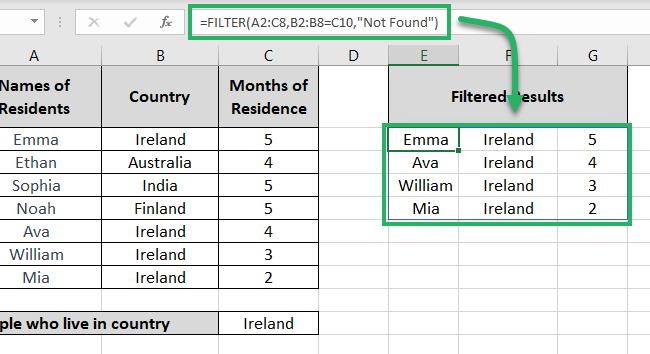
And there you go! The FILTER function filters out all the data for people who live in Ireland. And it is filtered out to a separate location (where the formula was typed).
Pro Tip!
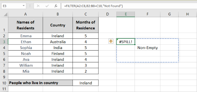
As the FILTER function returns an array of results, make sure you have enough empty cells to populate these results.
If not, you’d end up having the #SPILL Error like here😵
FILTER with multiple criteria: AND logic
In the previous example, we have run the FILTER function to find out the people who live in Ireland. This is one criterion only👀
But what if you want to apply multiple criteria simultaneously? For example, if you want to filter out the records for the people:
- Who live in Ireland; and
- Their residency months are 4 or more.
To apply these both criteria, we need to run the AND logic (with the multiplication operator). Take a look below🪁
- Write the FILTER function as follows:
= FILTER
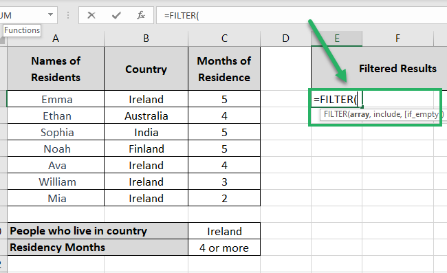
- As the first argument, specify the array from where the data is to be filtered i.e. A2:C8.
= FILTER (A2:C8,
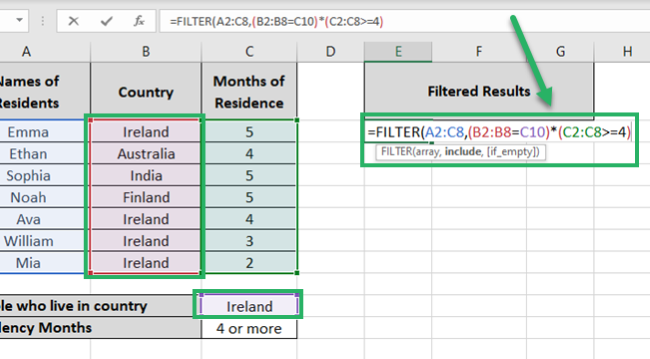
- As the second argument, write the criteria based on which records are to be filtered.
This time we have multiple criteria, where:
- The country is Ireland; and
- The residency months are 4 or more.
We will write it as follows:
(B2:B8=C10) * (C2:C8=>4)
Cells B2 to B8 contain the country. And Cells C2:C8 contain the residency months which should be equal to or greater than 4 (=>4).
Pro Tip!
The AND logic works on a simple science🎯
Both the criteria (B2:B8=C10) and (C2:C8=>4) are logical expressions. If they turn TRUE, the result would be 1, and if FALSE, the result would be 0.
As there is a multiplication operator in between, if any of the conditions turn FALSE, resulting in zero, the result would be zero.
(1 * 0 = 0)
So even if one logical test is true (1), if the other is false (0), the result would be 0.
- Set the if_empty argument to “Not Found” or any other dialog, as desired. You can set it to blank (“”) or omit it.
= FILTER (A2:C8, (B2:B8=C10) * (C2:C8=>4), “Not Found”)
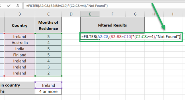
- Hit Enter now.
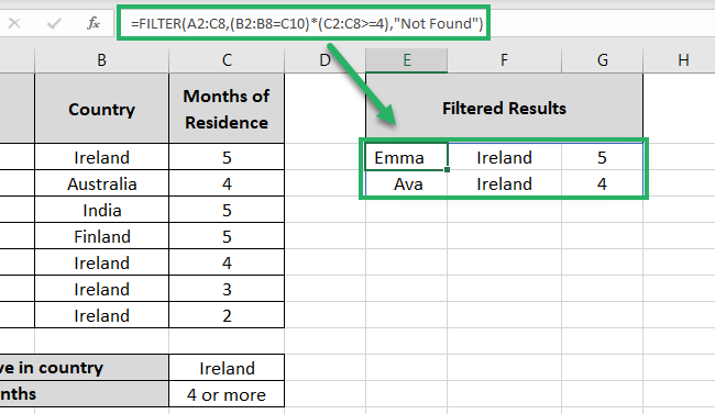
Okay wow! The FILTER function returns two entries. Both Emma and Ava are from Ireland and are residents for 4 or more months🚀
FILTER with multiple criteria: OR logic
Now, it’s time that we run the FILTER function with the OR logic. So with the same data set, let’s filter out the records for the people👨🏿🤝👨🏼
- Who live in Ireland; OR
- Their residency months are 4 or more.
To apply these both criteria with the OR logic, we need to run the FILTER function (with the addition operator). Take a look below.
- Write the FILTER function as follows:
= FILTER(
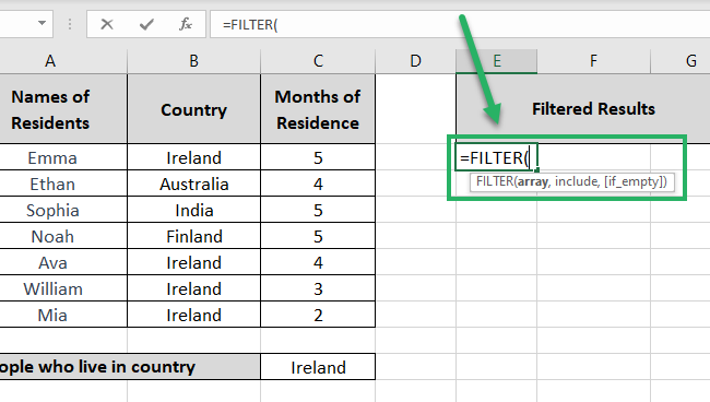
- As the first argument, specify the array from where the data is to be filtered i.e. A2:C8.
= FILTER (A2:C8,
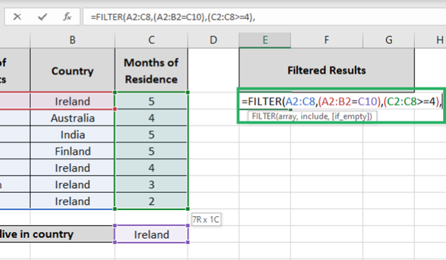
- As the second argument, write the criteria based on which records are to be filtered.
This time we have multiple criteria to be applied under the OR logic, where:
- Either country is Ireland; OR
- The residency months are 4 or more.
We will write it as follows✍
(B2:B8=C10) + (C2:C8=>4)
Cells B2 to B8 contain the country. And Cells C2:C8 contain the residency months which should be equal to or greater than 4 (=>4). And cell value for C10 is Ireland.
Pro Tip!
The OR logic works on the same science as the AND logic💁♀️
The formula stands on Boolean values (true/false).
Both the criteria (B2:B8=C10) and (C2:C8=>4) are logical conditions. If they turn TRUE, the result would be 1, and if FALSE, the result would be 0.
As there is an addition operator in between, unless both conditions are FALSE, the result won’t be zero.
(1 + 0 = 1)
So even if one condition is true (1), the result would be 1. And the FILTER function will not return the If_Empty value.
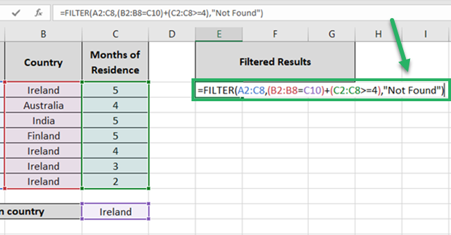
- Set the if_empty argument to “Not Found” or any other dialog, as desired.
= FILTER (A2:C8, (B2:B8=C10) + (C2:C8=>4), “Not Found”)
- Hit Enter now.
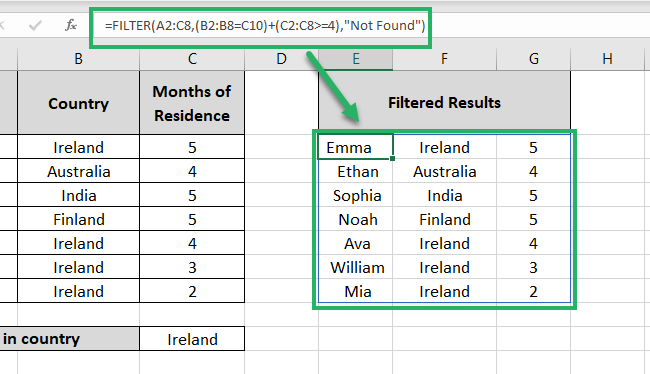
This time the list is long. The FILTER function extracts all the people who fit either criterion i.e. live in Ireland or are residents for 4 or more months😍
Easy to apply and great results – no?
That’s it – Now what?
If you didn’t know about the Excel FILTER function yet, this guide must have been your savior✨
In the guide above, we learned about filtering data using the FILTER function of Excel. You can use it simply or with multiple criteria under the OR & AND logic.
The FILTER function of Excel will help you sort your data and pick out the relevant stats in an instant.
Especially, when used to assist other major functions like the VLOOKUP, SUMIF, and IF functions, it eases your Excel jobs by a thousand times. Don’t know much about these functions? No worries.
Click here to sign up for my free 30-minute email course to help yourself learn these and many more amazing functions of Excel.
Other resources
If you enjoyed learning about the FILTER function of Excel, do not miss the chance to learn about other filtering tools of Excel too.
