How to Use the XMATCH Function in Excel: Step-by-Step
The XMATCH function is the successor of the MATCH function 🏹
And just as you guessed, it comes packed with many new advanced features that the MATCH function missed out on.
It is more flexible and versatile. Using the Excel XMATCH function, you can perform vertical and horizontal lookups. You can choose to perform an exact or approximate match.
And the best part – it comes with an in-built wildcard match mode. To learn more about what this robust function can do, continue reading the guide below 😎
Download our free sample workbook for this guide here to tag along with the guide.
Table of Contents
What is XMATCH?
The XMATCH function finds the relative position of a given value from a range of cells. More precisely, it is an enhanced (way enhanced) version of the MATCH function 💥
It is only available in Excel 365, and Excel 2021. The older functions of Excel do not support this function.
Pro Tip!
Here is the syntax of the XMATCH function 👇
XMATCH (lookup_value, lookup_array, [match_mode], [search_mode])
- Lookup_value is the value that is to be looked for.
- Lookup_array is the range of cells where the lookup value is to be looked for.
- Match_mode (optional) specifies if an exact or partial match is to be performed. It can be set to four modes:
-
- 0 (or omitted): Exact match
- -1: Exact match or the next smallest value
- 1: Exact match or the next largest value
- 2: Wildcard match
- Search_mode (optional) specifies the direction of the search. It can be set to four modes:
-
- 1 (or omitted): search from first to last.
- -1: Search from last to first.
- 2: Ascending binary search.
- -2: Descending binary search.
Simple XMATCH Excel formula
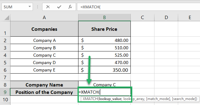
It’s time we see this robust function in action. Here we have the share prices for some companies 💹

Let’s write the basic XMATCH function to find the position of Company C in the list above.
- Write the XMATCH function as below:
= XMATCH (
- Write the lookup value (the value to be looked for) first.
= XMATCH (B8

We have referred to Cell B8 (which contains Company C) 🧐
- Refer lookup array (where the value is to be looked for) next.
= XMATCH (B8, A2:A6)

Company names sit in the cell range A2:A6. We have referred to the same as the lookup array 💡
- Hit Enter and there you go!

Company C is at the 3rd position in cell range A2:A6, and that’s what XMATCH returns.
This was the simplest application of XMATCH in Excel, and there’s much more to come 🚀
XMATCH formula examples
XMATCH outstands the simple MATCH function because of the additional search modes that it offers. Let’s explore these modes below💭
Example #1: Match mode
The MATCH mode in Excel helps you perform exact, partial, and wildcard character matches.
In the same example as above, let’s find the Company with a share price of $500 💸
There’s no such company in the data above so we will be going with an approximate match.
- Write the XMATCH function as below:
= XMATCH (C8
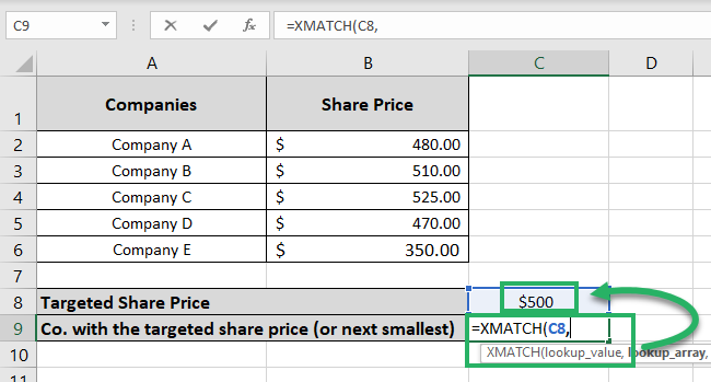
We have referred to Cell C8 (which contains $500).
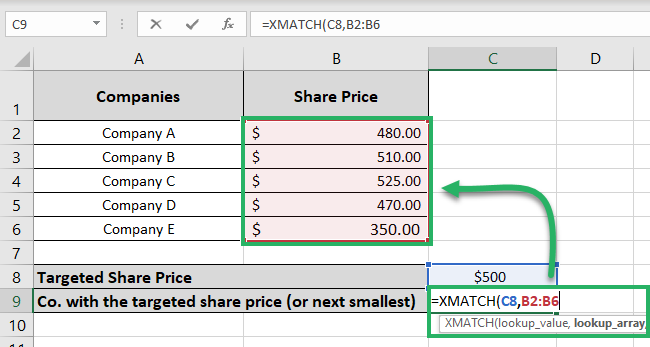
- Refer to the lookup array as B2:B6 (the range that contains share prices).
= XMATCH (C8, B2:B6)
- As the match mode, write -1.
= XMATCH (C8, B2:B6, -1)
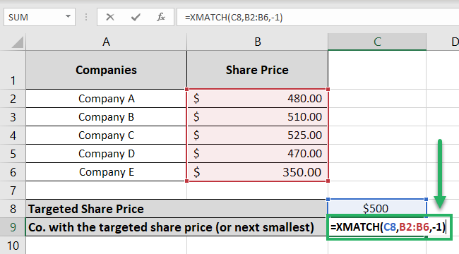
The match mode -1 finds the exact match first. If there is no exact match, it then looks for and returns the next smallest value 🔎
- Hit Enter.
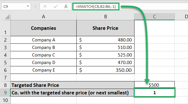
We get 1. On position 1 in the cell range B2:B6, we have a share price of $480 for Company A.
Our dataset has no Company with an exact share price of $500, and the next smallest share price is $480 – so yeah, it works 💪
Let’s try to run another match mode to find the share price next largest to $500.
- Change the match mode in the function to 1.
= XMATCH (C8, B2:B6, 1)

- Hit Enter.

This time the answer is 2. In the 2nd position in the range Cell B2:B6, we have $510 which is the next largest to $500 🤟
To perform an approximate match in numbers, use the match modes -1 and 1.
However, to perform partial matches in text, you can use the wildcard character match code of 2. The XMATCH function supports two wildcard characters (*,?).
Example #2: Search Mode with wildcard characters
The search mode of the XMATCH function tells it if a value is to be searched from the first or last. We will see this through the example below:

The image above shows the details of different awards won by the employees of a Company over the years 🏆
Using the XMATCH function, can we readily find the last award won by Abigail?
- Write the XMATCH function as below:
= XMATCH (D9
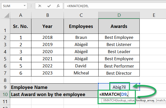
We have referred to Cell D9, which contains the name of the employee whose award we’re looking for 💁♀️
The spelling of Abigail in Cell D9 might seem a little odd to you.
Note that the spelling of the name Abigail varies in the list of employee names. Some instances have it named ABIGEIL, and others have it as ABIGAIL 😲
So we will perform a wildcard match by replacing the A and E with a question mark.
- Refer to the lookup array as C2:C7 (the range that contains the employee names).
= XMATCH (D9, C2:C7
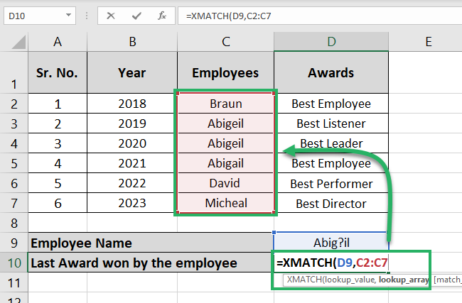
- As the match mode, write 2 (the wildcard mode) 📝
= XMATCH (D9, C2:C7, 2
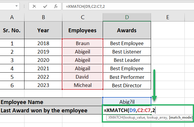
- Define the search mode as -1.
We want to find the last award won by Abigail. This means the search must be performed in a reverse manner (starting from the end of the list).
The search mode -1 will do that 🚴♂️
= XMATCH (D9, C2:C7, 2, -1)

- Hit Enter.
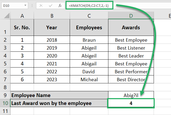
And we get a 4. The last time Abigail appears on the list of employees is in position 4.
That’s against the best employee for the year 2021 – the last award won by Abigail 🥇
Had written the same function with the search mode 1, the results would have been very different.
= XMATCH (D9, C2:C7, 2, 1)
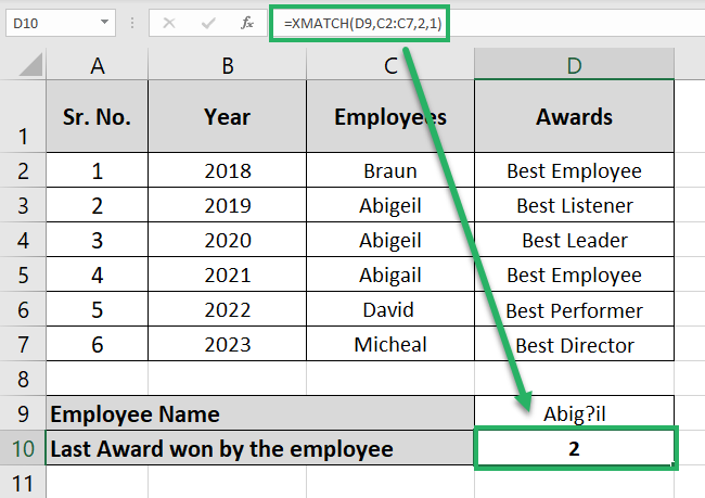
This time the answer is 2. The XMATCH function searches the list starting from the first to the last. So it returns the position when Abigail appeared for the first time on the list.
That’s on position 2 – Best Listener for 2019 🎧
Example #3: XMATCH with INDEX function
Match functions can act as lookup functions when combined with the INDEX function.
In the employee awards example above, the XMATCH function returned the relevant position of our lookup value 🙈
And we manually had to find the year and award won by Abigail in that position. The INDEX function will help us fetch that award and year automatically.
- Write the XMATCH function as below:
= XMATCH (D9
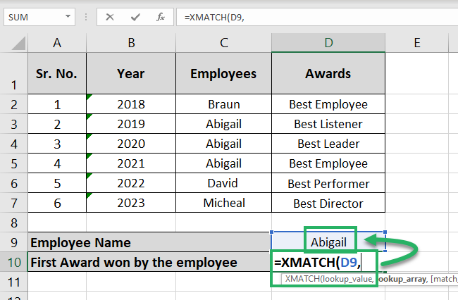
Referring to Cell D9 which contains Abigail. The spelling in the employee names list is now uniform so, no more wildcard characters ❌
- Refer to the lookup array as C2:C7.
= XMATCH (D9, C2:C7)
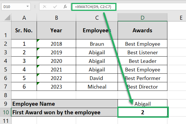
The XMATCH function returns the position of Abigail in the cell range C2:C7 🧠
- Wrap the above function in the INDEX function as follows:
= INDEX (D2:D7, XMATCH (D9, C2:C7))
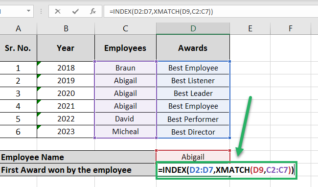
The first argument of the index function D2:D7 is the array from where the value is to be returned. We want the award type to be returned that sits in cell range D2:D7 🎯
The second argument of the INDEX function is the row number of the array whose value is to be returned. As the row number, we have nested in the XMATCH function.
- Hit Enter.

Oh wow! This time the result is not just a boring number. And you don’t need to go back looking into your data to find the value that corresponds to this number 😍
The INDEX function returns the value that lies on that position in the given array.
The result of the XMATCH function is 2 (we saw that above). So the INDEX function returns the second value of the array D2:D7.
This automatically brings you the first award won by Abigail 👆
Let’s now apply the same to find the year of the award too 📅 For that:
- Write the INDEX function as follows:
= INDEX (B2:B7, XMATCH (D9, C2:C7))
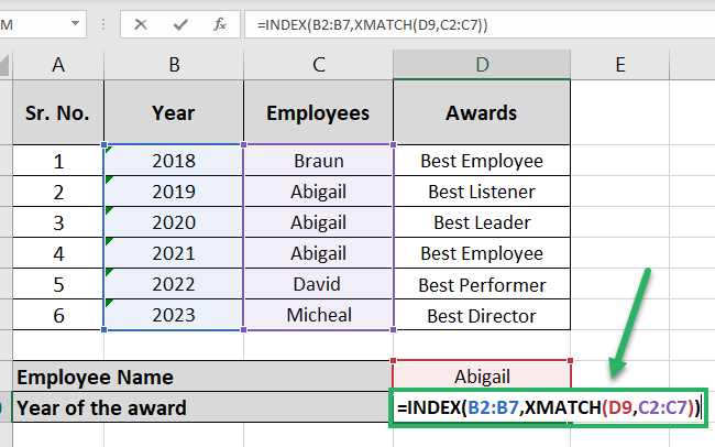
The function is just the same as it was above. We have only changed the first argument (array) of the INDEX function to B2:B7.
As we want to find the year when Abigail won the award we have set the array as the cell range that contains the years of awards (Cell B2:B7).
- Hit Enter to get the results.
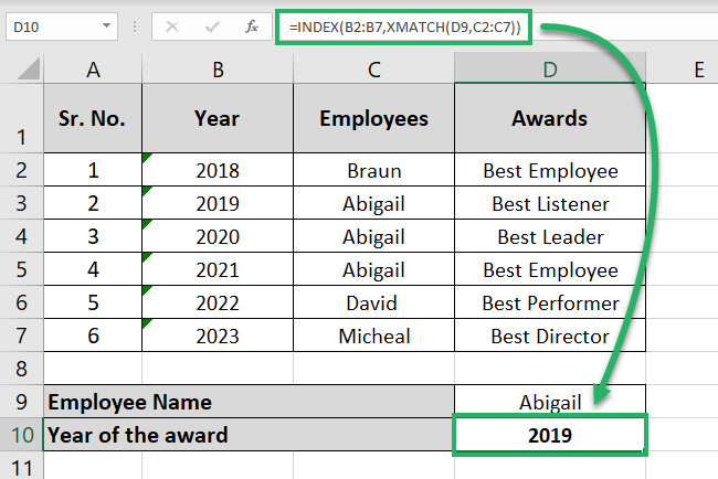
So now you know that the first award won by Abigail was the Best Listener award in the year 2019 ✌
That’s it – Now what?
Hope you enjoyed learning what the XMATCH function can do for you in Excel. It can look for a value in any dimension (both vertically and horizontally).
It can perform exact and partial matches and can also go on a wildcard character search mode. Such fun, no?
But hold on – that is just one function. The wide variety of Excel functions, tools, and features will have you amazed 😵
Some of my personal favorites from the Excel function library include the VLOOKUP, SUMIF, and IF functions.
Other resources
What is a match function without the INDEX function? You’ll make the best out of the XMATCH function when paired with the INDEX function.
