How to Count Cells With Specific Text Using a Formula
Counting cells with specific text in a worksheet is a task that one needs to perform on a daily basis to review large sets of data and extract information.
Luckily, Excel offers a variety of methods you can use to find text in your worksheet in seconds. In this tutorial, we will discuss and explain the easiest ways of counting cells with specific text in Excel.
Download our free sample workbook here to practice the topic firsthand. Let’s get started 🚀
How to Count Cells With Specific Text Using COUNTIF
One of the most popular methods of counting cells with specific text in Excel is to use the COUNTIF function. It allows you to conditionally count cells as you insert the target text string in arguments.
Microsoft Excel COUNTIF formula to count text values is given below:
where
range refers to the range of cells where the specific value is located at
text refers to the text string that is to be counted in the range.
Let’s now see an example where this formula can be applied.
Say, we have the following sample data set.
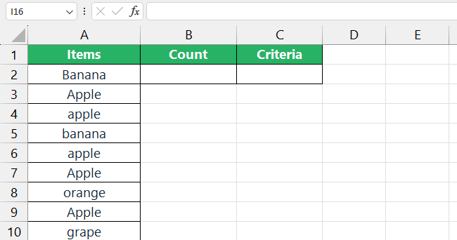
In column B, let’s calculate the number of times the word Apple appears in column A.
To do that,
Step 1) Select cell C2.
Step 2) Type in the word Apple 🍏
Step 3) Enter the following formula in cell B2
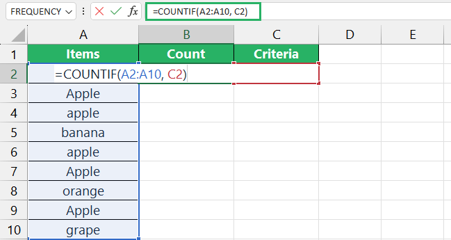
Step 4) Press Enter.
Step 5) The formula returns the count of the number of times the word Apple appears in the dataset.
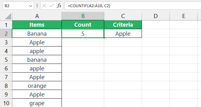
The formula returned the count 2 which is correct as Apple appears twice in the data set. But note that it counted all the cells that contained the same characters irrespective of their case.
This tells us that the COUNTIF function is not case-sensitive.
We will later see how you can count cells with case-sensitive data too.
How to Count Cells With Specific Values
We saw how you can find an exact match of your target string minus the case sensitivity in a data set using the count function. But what if your target string has a single different character at the start or it is positioned between two characters? 🤔
To deal with this scenario, we use wildcard characters.
All you need to do is place an asterisk (*) at the end of the string or cell reference that you pass to include the extra unknown character.
If the unknown character appears at the end of the string, write it as:
If the string appears between unknown characters, write the formula as:
Let’s see how to do this below with an example.
I want to find the word Apple in my data set but this time, my data has the word apple written in different ways.
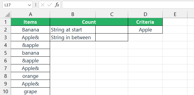
To find the word apple with an unknown character at the end,
Step 1) Type in the following COUNTIF formula in cell C2:
Step 2) Press Enter.
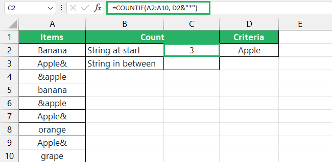
Make sure to add quotation marks at the start and end of the text parameter.
Now do the same for strings in between characters.
Step 3) Type in the following COUNTIF formula in cell C3:
Step 4) Press Enter.
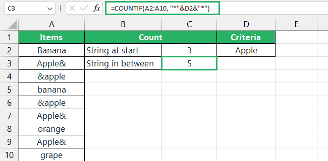
It’s that simple. Try it yourself now! 😃
How to Count Cells With Case-Sensitive Specific Text
Depending on the situation, you might need to count cells with case-sensitive values. Unfortunately, COUNTIF is not capable of dealing with this use case.
So we build our formula to find lowercase and uppercase text values depending on whether you want to find a partial or an exact match.
Let’s see how to find the two below.
How to Count Case Sensitive Cells with Exact Match
As the name suggests, exact match strictly compares the sample text with all the text cells in the given data range 📑
This means if your sample text is KL-34, it will check KL-34 and not kL-34 or KL,34. To count cells with specific text and ensure they are case-sensitive, we use the following combination of Excel formulas.
where,
EXACT function – an array formula – takes two arguments, text and range. It compares the sample text value with all other cells in the data range and returns an array of TRUE and FALSE for matched and unmatched values, respectively.
The double hyphen or double unary ( – – ) converts the TRUE and FALSE values to 1’s and 0’s as we need to return the count of text values.
SUMPRODUCT function adds up all the elements (1’s and 0’s) of the array returned by the EXACT function and displays as the number of counts.
Let’s now see its usage step-by-step through an example.
Say, we have the following sample data.
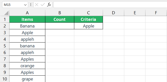
We want to find the word Apple in our dataset.
To do that,
Step 1) Select cell B2.
Step 2) Type in the following formula
Step 3) Press Enter.
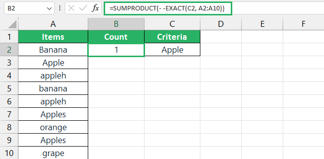
The formula returns a count of 1 which shows that it only considered the cell that exactly matched the text in the cell reference.
Easy, right?
How to Count Case Sensitive Cells with Partial Match
Unlike exact match, partial match looks for the targeted string anywhere in a cell for which we need to create a personalized formula that can be a little tricky. But don’t worry, we got you.
We will combine three different Excel functions to find a partial match of a string in a data range.
where,
FIND function searches for the target string in the entire data range and returns the index of the first character if found or a #VALUE! error. Our concern here is not the index of the first character – but any number instead of an error is our value here.
ISNUMBER function plays an important role as it converts any number returned by the FIND function to TRUE and FALSE and the double unary operator in between ( – – ) converts the TRUE and FALSE values to 1’s and 0’s.
SUMPRODUCT function takes in the array of numbers returned and sums them all up giving us our final count of instances where the string is found.
Let’s now see an example to understand how this formula works better.
We will use the same word as before – Apple – to search for in our data set.
To do that,
Step 1) Select cell B2.
Step 2) Type in the following formula:
Step 3) Press Enter
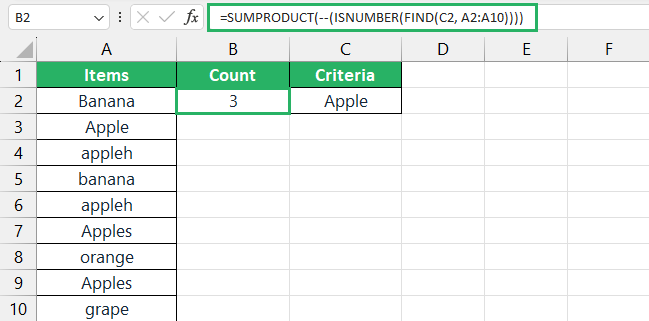
The formula returns the count 3 as the partial match of the string Apple.
Note that since the above combination of functions is for case-sensitive words, it only counts strings in the same case irrespective of their position.
Isn’t that cool? 🧐
Conclusion
All in all, counting cells with specific text is an important part of data analysis that gives you the leverage of manipulating and interpreting data in different ways.
The easiest way to achieve this is to use the COUNTIF and SUMPRODUCT functions. You can make different combinations like adding EXACT or ISNUMBER functions to get the desired result.
You can use the COUNTIF function for other purposes as:
How to Count the Number of Cells in a Range
We hope you enjoyed reading this article as much as we did creating it.
