How to SUM by color in Excel:
Step-by-Step Guide
Most of you know how to get the Excel SUM. It’s one of the most basic Excel functions.
What most people don’t know is that you can get the Excel SUM by color, too 🤩
There is no built-in function for this but it doesn’t mean Excel can’t 😉
Today, you’re in for a colorful, in-depth lesson on how to SUM by color in Excel.
Let’s go!
Table of Contents
SUM cells by color with filter and SUBTOTAL
The contribution made by association members to a project is displayed in the Excel table below 💰
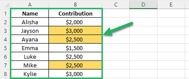
The amount that has yet to be collected is indicated in the highlighted cells.
Let’s say you want to know the total of the cells that have been highlighted.
You can find the total value of all the colored cells by following the steps below 👍🏻
- Enter an equal sign in cell B9 and select the SUBTOTAL function.
=SUBTOTAL(

- Enter 9 as the function number. The number 9 is the function number of the SUM function.
Then, your formula is;
=SUBTOTAL(9
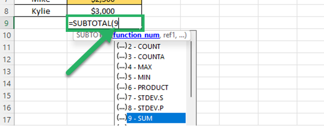
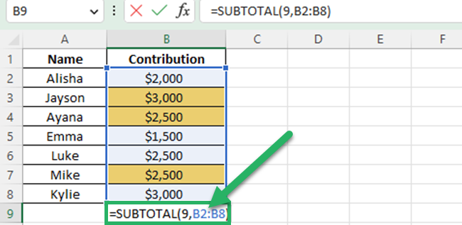
- Then, select the cell range of the values and close the parentheses.
You can see the following formula in your formula bar.
=SUBTOTAL(9,B2:B8)
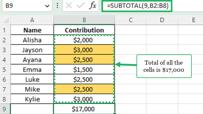
- Press the Enter key and you will get the total of all the cells.
- Select any cell or the whole data table and click the Filter icon. You can get the Filter icon from the Data ribbon.
Pro Tip:
You can select any cell of the data table and press “Control + Shift + L” to get the Filter command quickly.

- Now, filter the cells based on color. To do that, first, expand the drop-down menu of “Column B”. Then, expand the filter by color and go to the Filter by cell color. Next, select the color of the colored cells.
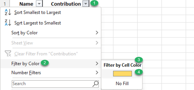
Excel will filter the cells based on the selected color.
Now, the SUBTOTAL formula will show the sum of the visible cells 😍
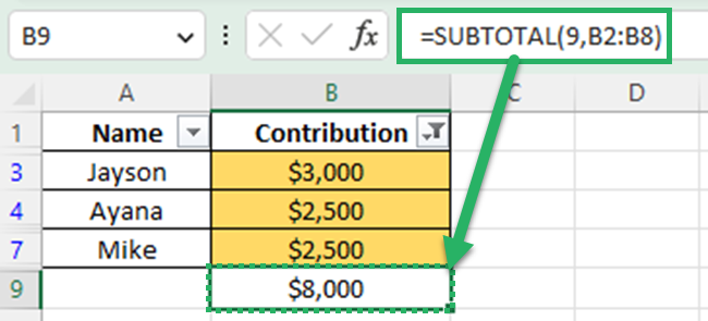
If you enter 2 for the function number of the above formula, Excel will count cells based on cell color 🥳
SUM cells by color with VBA code
Even though there are no in-built Excel functions for SUM by color in Excel, you can create a user-defined function using VBA.
So, with the help of VBA code, you can create a custom function to summing colored cells.
You can follow the below steps for that.
- Go to the Developer Tab and click Visual Basic.

- Click the Insert Tab of the “Microsoft Visual Basic for Applications” dialog box and go to the “Module”.

- Enter the below VBA code as a new module code.
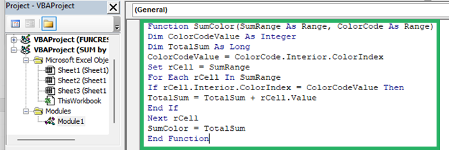
- Close the VBA Editor.
- Apply the custom function that you have created.
=SumColor(SumRange,ColorCode)
After selecting the SumColor function, select the color cells as the sum range for the first argument.
Then for the second argument, select a cell that has the same background color as the color that you want to add.
So, in this case, you can use the above color function as follows.
=SumColor($B$2:$B$8,D2)
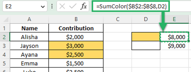
The SumColor will get the sum based on color 🤩
SUM cells by color using GET.CELL
You can get the sum of the colored cells using the GET.CELL function 🤔
GET.CELL function is an undocumented function in Excel. That means you cannot see it in the functions list.
GET.CELL function helps to get the cell information.
Follow the below steps to get the sum of the cells which are matching to the given color code.
- Use the type number 38 of the GET.CELL function and create a named range for column B. The type number 38 helps to get the cell background color code.
So, select Cell C2 and go to the Formulas tab.
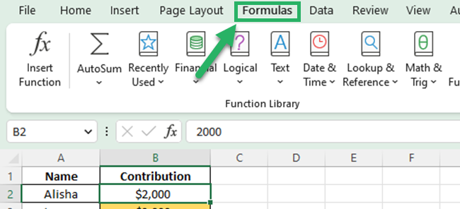
- Click the Name Manager icon to open the Name Manager dialog box.

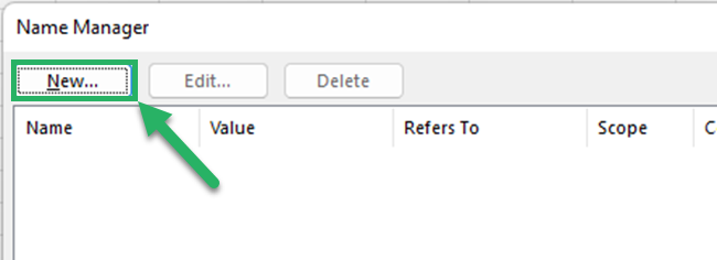
- Click the “New” button from the Name Manager dialog box.
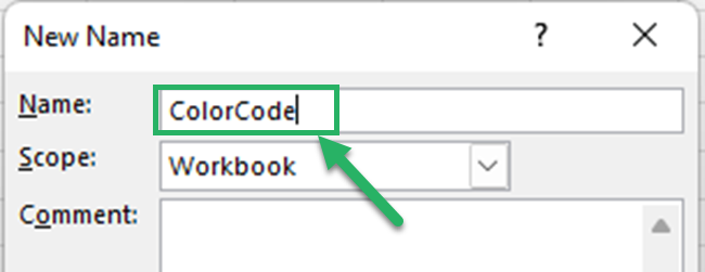
- In the new name dialog box, enter a name. You can enter a name like “ColorCode”.
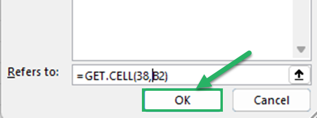
- In the “Refers to field”, enter the GET.CELL function to get the color code of the cell. GET.CELL function arguments are the Type number and the reference. In this case, to get the background colors, enter 38 as the type number and give the cell reference to cell B2.
=GET.CELL(38,B2)

- Click “OK” and close the Name Manager dialog box.
- Create a new column next to column B as the color codes.
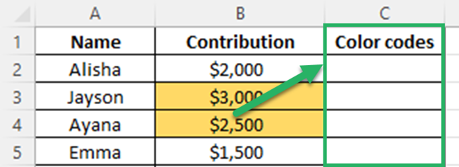
- Enter the following formula in the Color codes column (column C)
=ColorCode
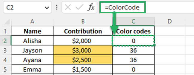
You will get 0 for the no-fill colored cells and a color value of 36 for the cells that look orange color.
- Now, use fill color and enter all the colors you have used in another column as in the below image.

Get the SUM of the colored cells
Use the SUMIF function to get the sum value based on the fill color of the adjacent cell (Cell F2).
It will get the adjacent colored cell as the criteria for the formula.
You can apply the same formula for the below cells as well.
=SUMIF($C$2:$C$8,Color_code,$B$2:$B$8)

In Excel-language, 1 means TRUE. 0 means FALSE.
That’s it – Now what?
Good work! Now you know how to get the SUM by color in Excel 👍
As you’ve learned, there are three different methods for calculating the SUM, based on color index values.
Among the three methods, VBA stands out because it allows you to create a user-defined function. And this is not only true for SUM by color, but a whole lot more 🚀
Want to get started with Excel VBA? 😀
Sign up for my FREE Excel Advanced User Training where you’ll learn the basics of VBA editor and how to write your first macro from scratch.
I promise you, it’s not as hard as you think 🤗
Other resources
You can refer to our VBA articles like “Learn VBA in Excel” and “VBA data types” if you wish to write your own VBA code to add up the colors of the cells.
Our articles on the SUMIF function and the SUBTOTAL formula will be quite useful as you practice this lesson 😊
