How to Highlight a Row in Excel (All Scenarios Shown)
Highlighting rows in Excel allows you to quickly identify key information in your data and make analysis a quick process 😃
Adding color to your worksheet also improves readability and makes it look more appealing. There are various techniques for highlighting rows in Excel that work for different purposes.
In this guide, we will look at different ways of highlighting rows in Excel. Download our sample workbook here to tag along with the guide and get hands-on practice.
How to highlight rows manually?
The most obvious method is to manually highlight each row in your data set. This can be tiresome if you have a huge number of rows to cover but it works well for less number of rows.
Say, we have the following sample data where we want to highlight one cell after the other in yellow color 🟨

To do that,
Step 1) Select alternate rows of your data set.
Step 2) Right-click the rows.
Step 3) Select the Format Cells option from the dropdown list.

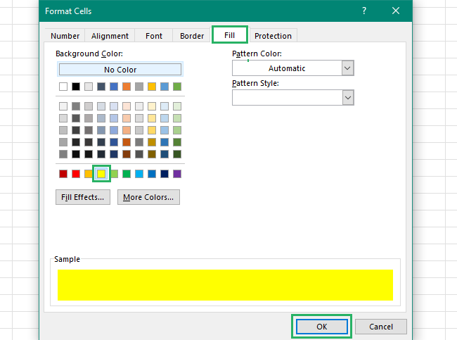
Step 4) The Format Cells dialog box will appear.
Step 5) From the dialog box, select the Fill tab.
Step 6) Select the color you want to apply to your rows, – in our case yellow.
Step 7) Click Ok 😃
You can also use an easier approach to the same solution.
Step 1) Select the alternate cells.
Step 2) Go to the Home tab and click on the small down arrow next to the Fill button in the Font group.

Step 3) Select the color you want to apply from the dropdown that appears.
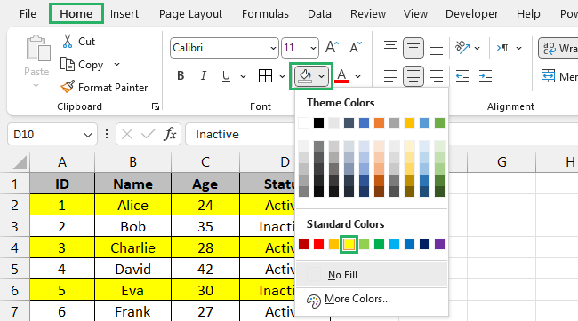
The selected cells will be highlighted in the copied color 🎨
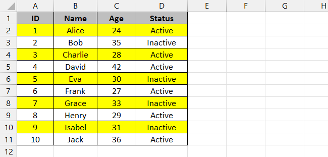
That was easy, no?
How to highlight rows using Format Painter?
You can also use the Format Painter feature to highlight rows in Excel. Format Painter comes in handy when you already have a data set with the desired format and you want to copy it to another place.
This is most helpful when you have a large data set and want to transfer the format without the actual cell value of the set. So selecting a format painter with your active row being colored in red will paste the red color to the next cell to be selected 🚩
We will use the same sample data as above. We want to copy the format of the highlighted rows and paste it into the remaining rows in our data set.

To do that,
Step 1) Select any highlighted row or cell.
Step 2) Go to the Home tab and select the Format Painter button from the clipboard section.

Step 3) The selected format will be copied to the clipboard 📄
Step 4) Now press CTRL and select the cells you want to transfer the format to.
The selected rows will be highlighted in the selected color:
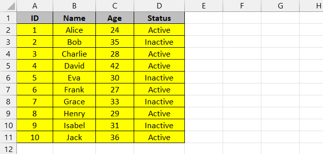
How convenient was that? Try it now!
How to highlight rows using Find & Replace?
Another fun and easy method of highlighting rows in Excel is to use the Find & Replace feature in Excel. This is the best option to use when you want to highlight rows containing the same value.
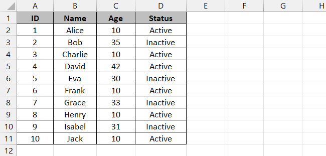
Say, we have the following sample data containing multiple instances of the age 24. We want to highlight all rows containing the same value in blue color 🟦
To do that,
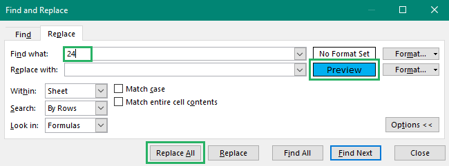
Step 1) Press CTRL + H on your keyboard or go to the Home tab and click on the Find & Select button from the Editing section.
Step 2) In the Find what box, enter the number 24 to be found.
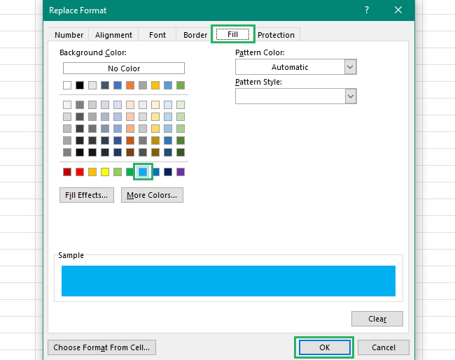
Step 3) In the Replace with box, click on the Format button and select the highlight color you want.
Step 4) Press Ok,
Step 5) In the Find & Replace dialog box, click on the Replace All button 🔁
All the cells with the entered value will be colored in blue as:

Pretty cool, right? 🤓
How to highlight rows using conditional formatting?
If you want to highlight the rows in your data set based on a set of conditions, you need to use conditional formatting.
This is a rather advanced level of Excel but it’s very easy once you get a hold of it. Let’s see how it’s used below 🔽
Highlight rows based on a condition
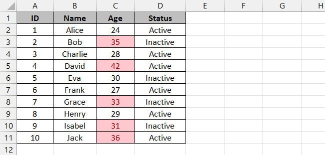
We will use the same sample data as used earlier. We want to color all rows in our data set that are greater than 30 using a simple rule.
To do that,
Step 1) Select your data set.
Step 2) Go to the Home tab and select the Conditional Formatting button from the Styles group 🏠
Step 3) Select the Highlight Cells rule from the options and then the Greater than option.
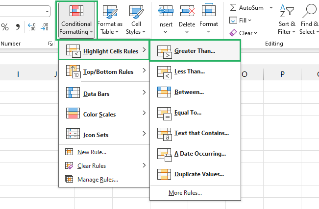
You can also select the Top/Bottom rules if you want to highlight cells based on their position in a range of cells. Or if you want to use a formula for a specific purpose, you can use the New Rule option that lets you create a new condition.
Step 4) The Greater Than dialog box will appear on the screen.
Step 5) Enter the threshold value for your formatting – in our case 30 and select the highlight color.
Step 6) Press Ok.

The result cells that meet the condition will be highlighted as:

Easy, no? 😃
Highlight rows based on text criteria
Let’s now see how to highlight rows in your data set based on the text they contain.
We have the following sample data and we want to highlight all rows that contain the word ‘Delivered’. We will use an Excel formula to do that.
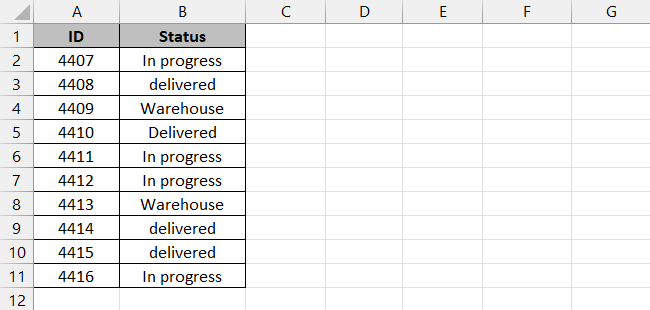
To do that,
Step 1) Select your data set.
Step 2) From the Conditional Formatting option, select New Rule ✅
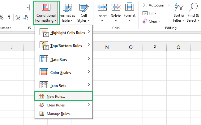
Step 3) The New Formatting rule dialog box will appear on the screen.
Step 4) From the Select a rule type, select ‘Use a formula to determine which cells to format’.
Step 5) Under the ‘Format values where this formula is true’ bar, enter the SEARCH formula as:
We could also use the Find & Replace method here but it is case-sensitive. Our data contains entries in both uppercase and lowercase and Find & Replace might not be our best bet here. So instead we use the case-insensitive SEARCH function that looks for the word in both cases.
Step 6) In the Preview option, click Format and select the color you want to highlight cells in.
Step 7) Press Ok.

The conditional formatting rule will color all the cells in the selected range that contain the word delivered 🖌
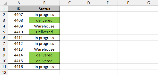
How cool is that? You can do this for any other word or string of text. Try it now!
Highlight rows with specific date criteria
You can highlight rows containing a particular date the same way you highlighted rows with specific text. The only difference is the formula being used.
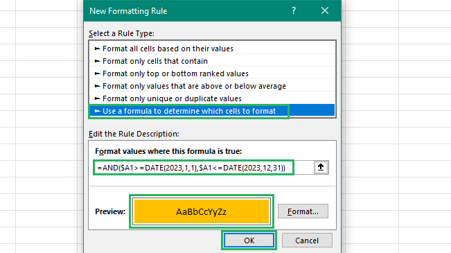
Say, we have the following sample data that consists of dates when different products were ordered. we want to find all the products ordered in a certain time period 📆
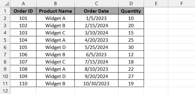
To do that,
Step 1) Select your entire data range.
Step 2) From the Conditional Formatting option, select New Rule.

Step 3) The New Formatting rule dialog box will appear on the screen.
Step 4) From the Select a rule type, select ‘Use a formula to determine which cells to format’.
Step 5) Under the ‘Format values where this formula is true’ bar, enter the following formula:
Step 6) In the Preview option, click Format and select the color you want to highlight rows in 🎨
Step 7) Press Ok.
The conditional formatting rule will color all the cells in the selected range that contain any date in the specified range.
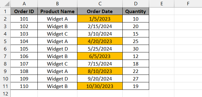
That’s so useful. Conditional formatting makes things so much easier 🧐
How to highlight rows using VBA?
If your data set is complex or large, you can use VBA to highlight cells based on a condition for you. This method requires creating and running a macro but it’s very straightforward.
We will use the same sample data as above. We want to highlight the cells that have a value greater than 30 in blue and cells with a value less than 30 in yellow 🟨
To do that,
Step 1) Press Alt + F11 on your keyboard to open the Visual Basic editor.
Step 2) In the editor, click on the Insert tab and select the Module option.
Step 3) Copy and paste the following code into the Module.
Step 4) Once done, close the Visual Basic Editor ❌
Step 5) Press Alt + F8 on your keyboard to open the Macro dialog box.
Step 6) Under the Macro name, select ColorCells.
Step 7) Press Run.

The rows in your range meeting the condition will be highlighted in blue and yellow respectively.
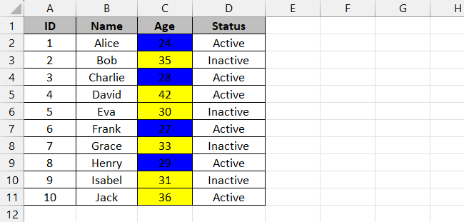
Isn’t this fun? Use VBA now! 😃
Conclusion
In this tutorial, we saw different scenarios to highlight rows in Microsoft Excel. We saw how to highlight cells manually and using Format Painter and find and replace 🔁
We also saw how to perform the same task using an advanced technique like VBA and conditional formatting. Conditional formatting offers a variety of options that you can use to highlight cells.
You can color them with different conditions like finding a certain piece of text, a date format, a number, etc. To learn more about conditional formatting and Excel tips, read our articles below.
How to Use Conditional Formatting to Highlight Text in MS Excel
Learn VBA in Excel: These 11+ Tutorials Teach You VBA in 20 Hours
How to Fill Color in Excel Cell Using a Formula
We hope you enjoyed reading this article as much as we did crafting it! 🤗
