How to Perform Linear Interpolation in Excel (Easy)

Interpolation means to estimate data points for two given variables.

A linear relationship between two variables refers to the relationship where the change in one variable is rooted in the proportional change in another variable.

It can be drawn up as a straight-line graph that moves predictably since when one variable increases/decreases, the other variables also increase/decrease at the same rate.

Within such variables that bear a linear relationship to each other, interpolating a variable value between two known data points is called linear interpolation 📈

I know your next question – can we perform it in Microsoft Excel? Obviously, we can, and this guide will teach you all the possible methods to do so.

So, grab your free practice workbook for this guide here and continue reading.

Table of Contents

Interpolation using Simple Mathematics

Interpolation is all about a simple formula, and you can do it manually by running some simple mathematics, too.

The formula is as below:

• Where Y is the dependent variable (the value of which depends on X).
• And X is the independent variable.

Putting this formula into action is super simple, let’s take an example to understand 🎬

For example, we have some data for the time and distance variables. That is how much time it takes to travel how much distance. Where time is variable (x) and distance covered being dependent on time is variable (y).

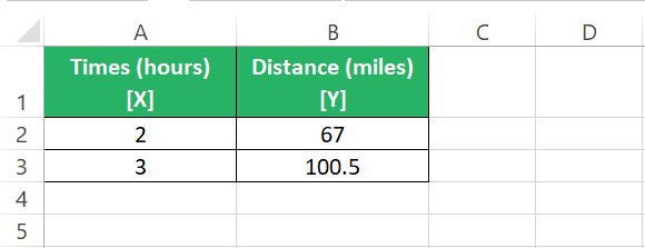
Looking at the data, I can see it takes 2 hours to cover 67 miles and 3 hours to cover 100.5 miles 🚲

If I quickly plot a graph out of these data points in Excel, it would look like this:

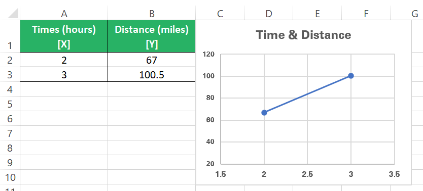
From this graph, I know the distance covered in 2 hours, and in 3 hours. But what is the distance covered in 2.5 hours?

2.5 is a point that lies on this straight-line graph in between the two data points that we have. It comes here 🏸

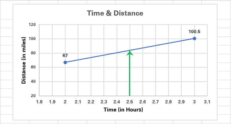
Finding the y value (distance) for an x value (time) that lies on a straight line between two points is what we call linear interpolation. 

Pro Tip!

Interpolation means estimating the value of a variable between two given data points. For example, we know the distance covered in 2 hours and in 3 hours.

Finding the distance covered in 2.5 hours (that lies between 2 and 3 hours) is called interpolation. Had we been estimating the distance covered in 4.5 hours (that lies outside the given data points), it would be extrapolation of data. 

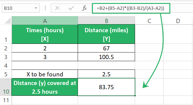
To find this mathematically in Excel, follow these steps.

Step 1) Find the difference between both the given values for the Y variable i.e., (Y2-Y1).

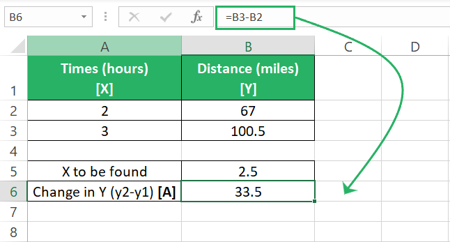
Step 2) Find the difference between both the given values for the X variable i.e., (X2-X1).

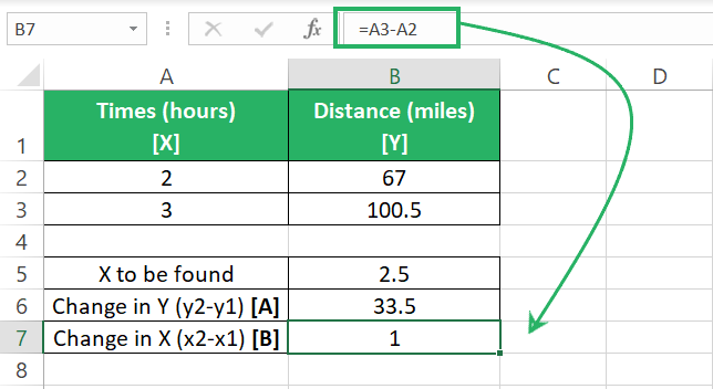
Step 3) Divide the difference in the Y variable by the difference in the X variable to find the rate of change in Y caused by the change in X.

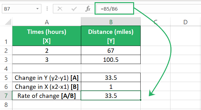
Step 4) Calculate the difference between the interpolated X and the first value of X (x1).

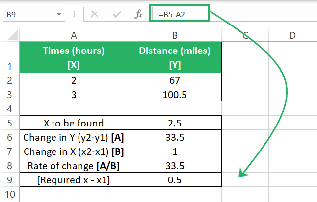
Step 5) In the next step, multiply the difference between the interpolated X and X1 by the rate of change in Y.

Step 6) Add the value of X1 to it.

Pro Tip!

All in all, we have applied the whole linear interpolation formula given above as follows:

It is just broken down in the steps above for a better explanation.

This gives us the value of Y for interpolated X of 2.5 as 83.75.

In other words, interpolating based on the given data points, 83.75 miles long distance would be covered in 2.5 hours.

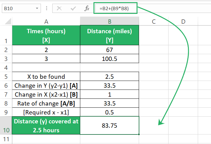
Hope this explains how interpolation works 😎

Interpolation using the FORECAST.LINEAR function

What is the purpose of using Excel if you’re not using Excel functions? The same interpolation that we did mathematically above can be done using the FORECAST.LINEAR function of Excel 🚀

Continuing with the same example, as above, we can interpolate the distance covered in 2.5 hours using the FORECAST.LINEAR function as follows:

Step 1) Write the FORECAST.LINEAR function as follows:

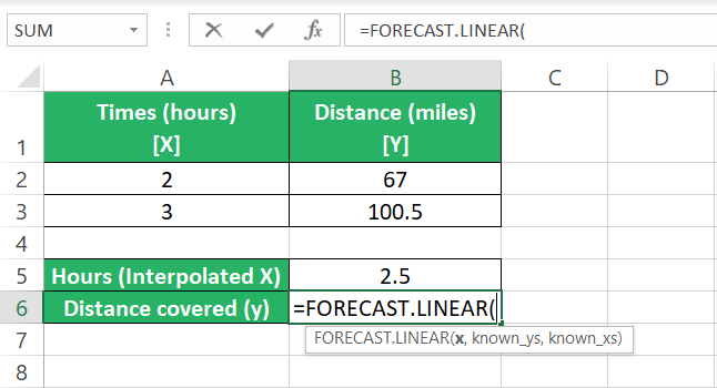
Step 2) As the x argument, refer to the cell containing the value for interpolated x.

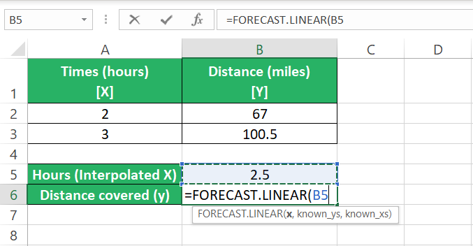
Step 3) Next, refer to the value of known-ys (the known data points for the variable y).

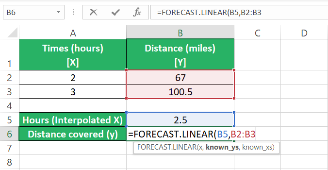
Step 4) For the third argument, refer to the value of known-xs (the known data points for the variable x).

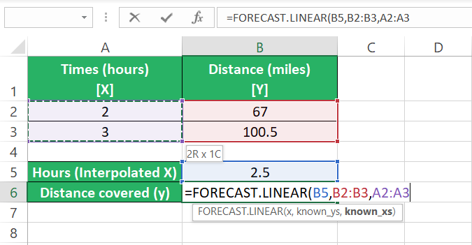
Step 5) All done. Press enter.

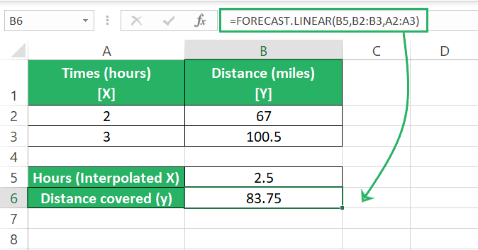
The FORECAST.LINEAR function also returns 83.75 miles as a result.

Same as we calculated above. Hence, proved, that if you have 2 data points for each of the x and y variables, you can use the FORECAST.LINEAR function of Excel to simplify your linear interpolation like that.

Interpolation for more than 2 values of X&Ys

Interpolation is not only about 2 values for each of the variables, but it can also have more than 2 values. 

For example, assume we have the following dataset for time and distance covered ⌚

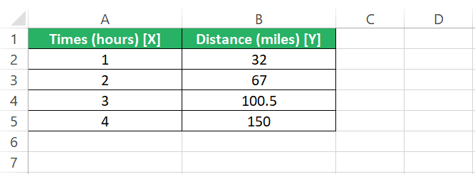
The dataset has expanded to include more data. We now also know the distance covered in 1 hour and 4 hours.

Using this data if you want to interpolate the value of distance covered for 2.5 hours, you can do it in two ways. 

Find the values of x1,x2,y1 and y2

What is the difference between the above dataset of two values and this dataset? Some additional data points.

Eliminate that difference, and the interpolation would be the same as before. To do this, we need to find the value for x1, x2, y1, and y2 🔢

Pro Tip!

Basically, x1 represents the value immediately next smaller than the interpolated x, and x2 represents the value immediately next larger than the interpolated x.

Y1 and y2 are the data points corresponding to x1 and x2. We will perform a quick exercise to find the value next smaller and bigger to the interpolated x.

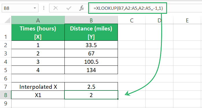
Step 1) Use the XLOOKUP function to find the value of x1 as follows:

• The first argument is the lookup value which is that of interpolated x i.e., 2.5.
• The second argument is the lookup array where the value is to be looked up. Referred as the dataset for known_xs.
• The third argument is the return array from where the value is to be returned. Referred as the dataset for known_xs again.
• Omit the optional fourth argument for if_not_found.
• The fifth argument is the match mode that we have set to -1. It tells Excel to look for the interpolated x (of 2.5), and if not found, return the next smallest value.
• The sixth argument is the search mode that we have set to 1. It tells Excel to start the search from the first to the last value.

The XLOOKUP function looks for the value 2.5, and since it is not present there, it returns the next smallest value of 2.

Step 2) Again, write the XLOOKUP function to find x2.

Everything remains the same except for the match mode that we have set to 1 this time so that Excel returns the next largest value  for X.

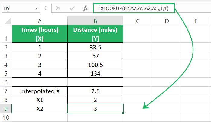
And Excel correctly returns the value for X2 as 3 which is next largest value to 2.5.

Step 3) We will use the XLOOKUP function again to find the value for Y1.

• We want to look up the y value that corresponds to x1  so, the lookup value is set to x1 i.e., 2.5.
• The lookup array where the value is to be looked up is set up as the known_xs.
• The return array from where the value is to be returned is set up as known_ys.
• Omit the optional fourth argument for if_not_found.
• The match mode is set to exact match (0).
• Omit the search mode argument too.

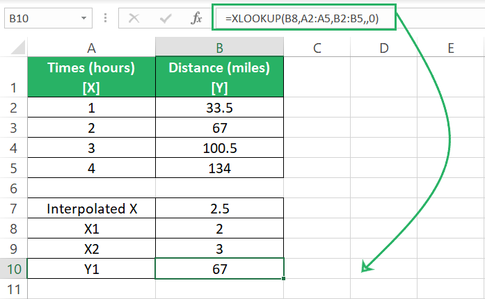
Excel rightly finds the value of Y that corresponds to X1 as 67.

Step 4) Again, use the XLOOKUP function to find the corresponding value of Y for x2.

Nothing changes really except for the lookup value  which is now set to X2 🧐

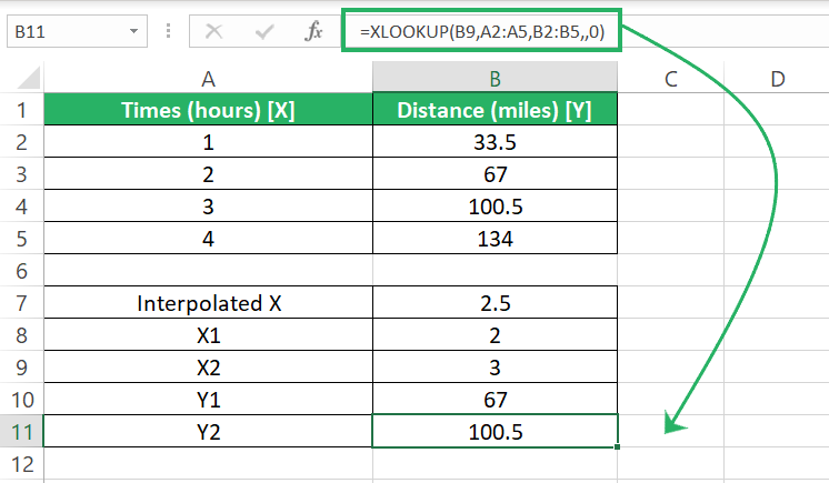
Y2 comes out as 100.

Step 5) Here onwards, you may apply the FORECAST.LINEAR function as below to find the distance covered in the interpolated 2.5 hours.

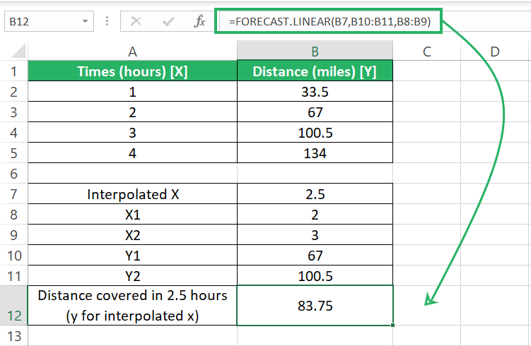
Or elsewise, you may use the mathematical formula discussed above to find the interpolated value.

The answer would remain the same 💡

Use the entire dataset

The other method to estimate the interpolated value of y for x when you have multiple data points is to simply use the FORECAST.LINEAR function for the whole dataset.

Step 1) Write the FORECAST.LINEAR function as follows:

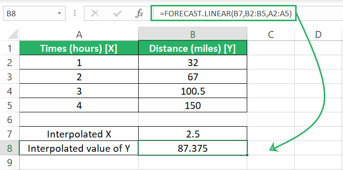
The FORECAST.LINEAR function returns the distance as 87.375 this time.

By now, you know how to interpolate variables from your dataset in Excel for any data type. Quickly and accurately 💪

Conclusion

Linear interpolation is an important but one of the many statistical techniques to forecast data in MS Excel. There are other methods too that you might want to use to draw a linear relationship between two variables.

Interested to know more? Hop on to my following advanced Excel tutorials to learn all about these.

• How to do Linear Regression in Excel: Full Guide (2024)
• How to Use the Excel FORECAST Function Step-by-Step (2024)