How to Use the OFFSET Function in Excel
– 3 Examples (2024)

The OFFSET function returns a range of cells that is located a specified number of rows/columns away from a specific cell.

While this has no use on its own, it’s extremely useful in specific scenarios when combined with other functions.

The OFFSET function can be hard to understand without visualizing it, so let’s just dive in💡

To follow along with this guide, I suggest you download my sample file here.

Step 1: The reference argument

Have a quick look at the OFFSET example in the picture below.

I want you to return the salary of the person 2 rows below Abigail. So, 2 rows below row #2 in column C. And put it in E2.

Let’s get started👍

The syntax of the OFFSET function consists of 5 arguments, and 2 of them are optional.

The first part of the syntax is the reference argument.

The reference argument is the starting cell from where you want to go X rows down/up or Y columns right/left.

Write:

=OFFSET(C2

So, to go 2 rows down from Abigail’s salary, you need to start in C2.

And as always, end the argument with a comma to let the OFFSET function know you’re moving to the next part of its syntax.

Step 2: The rows argument

The rows argument tells the OFFSET function the vertical location of the range you want to return (down/up)

You want to return something 2 rows below the starting reference.

So, write 2.

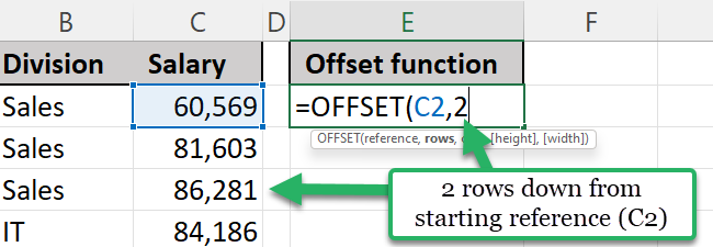
The rows argument works with both positive numbers and negative numbers.

– (minus) is up
+ (plus) is down

Your OFFSET function should look like this by now:

=OFFSET(C2,2

Almost done already⏱️

Step 3: The columns argument

The columns argument tells the OFFSET function the horizontal location of the range you want to return.

In this example, the cell you want to return is located in the same column as the starting reference.

So, you actually don’t want to tell the OFFSET function to go any columns to the left or right.

But you do need to tell OFFSET that you want to stay in the same column.

So, write 0.

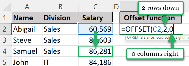
Your OFFSET function should look like this:

=OFFSET(C2,2,0

Now, if you wanted to return something that’s not in the same column as the starting reference you could write a positive or negative number instead.

– (negative) is left
+ (positive) is right

So, if you wanted to return the ‘Division’ from column B instead, you’d have to write -1.

Write and end parenthesis to close the function.

So the final function should look like this, for returning the salary 2 rows below Abigail’s (no column change).

=OFFSET(c2,2,0)

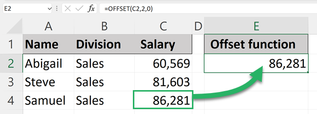
And that’s exactly what it does.

The OFFSET function returns the contents of the cell 2 cells below the starting cell.

Beautiful, right?

“But Kasper… What about the other 2 arguments?

They’re optional😊

Let me explain…

Step 4: Height and width arguments (optional)

The height and width arguments are only used to return a range of multiple adjacent cells.

In the above example, where you wanted to return the content of a single cell, the height and width arguments are useless.

Height = number of rows
Width = number of columns

The top left part of the range, is the ending point after the first 3 arguments.

And as earlier:

– (negative) is left
+ (positive) is right

Here are two OFFSET function examples that focus entirely on the height and width arguments:

The left OFFSET example

=OFFSET(A1,1,2,2,-2)

It starts in cell A1, then goes 1 row down and 3 columns to the right. We’ll call this point B.

From there it starts selecting a range that is 2 rows high (going down from the top of point B) and 2 columns wide (going left of B).

The right OFFSET example

=OFFSET(A1,2,3,1,-2)

It starts in cell A1, then goes 2 rows down and 3 columns to the right. We’ll call this point B.

From there it starts selecting a range that is 1 row high (going down from the top of point B) and 2 columns wide (going left of B).

“How’s that useful?”

That’s a good question.

On its own, it isn’t🤷

But you can use the offset function to return a range of cells into another function – and that’s where the magic starts.

Example: OFFSET dynamic range (COUNTA)

A dynamic range is a range that automatically expands to the amount of data within it.

When you combine the OFFSET function with the COUNTA function, you create a dynamic range.

This is especially useful when combined with a ‘named range’ to make a ‘dynamic named range’.

Let’s dive in🤿

Understanding dynamic named ranges

The normal syntax for the OFFSET function is:

=OFFSET(reference, rows, columns, [height], [width])

Replace the height argument and the width argument with the COUNTA function. Like this:

=OFFSET(reference, rows, columns, COUNTA(range), COUNTA(range))

As you can see, the 1st COUNTA function replaces the height argument, and the 2nd COUNTA function replaces the width argument.

So, this is the syntax you need to use:

=OFFSET(reference, rows, columns, COUNTA(range))

Step 1: Set starting reference

To start this OFFSET formula, make a cell reference to where the dynamic range should start:

=OFFSET($A$2

IMPORTANT:

Do remember to lock all references used in this OFFSET formula🔒

Step 2: Set rows and columns arguments to 0

Add 0 for the number of rows and columns.

=OFFSET($A$2,0,0

Step 3: Replace height argument with COUNTA function

Add the COUNTA function instead of the normal height argument.

=OFFSET(A$2$,0,0,COUNTA($A:$A))

This tells the OFFSET formula how tall the range should be to match the data in it.

It does so by counting the number of non-empty cells in the specified range using the COUNTA function. The count is returned to the OFFSET function as the height argument – the number of rows the range should include.

Step 4: Open Name Manager

Open the ‘Name Manager’ from the Formulas tab.

Step 5: Create a new named range

Click the ‘New’ button to create a new named range.

Step 6: Insert OFFSET formula

Copy the OFFSET formula you made before into the ‘Refers to’ field.

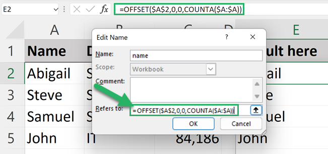
Click OK and close the Name Manager.

That’s it👏

Now, you can use your new dynamic named range in your Excel formulas.

A ‘dynamic named range’ is great for keeping your ranges tight, so they don’t include any empty cells that slow down your file.

But the ‘dynamic named range’ truly shines when used as the source in a drop-down list☀️

Example: OFFSET and MATCH function

The combination of OFFSET and MATCH is a lookup formula just like VLOOKUP or INDEX MATCH.

Especially like INDEX MATCH!

MATCH looks for a value and returns the row number of the found value to the OFFSET function. And the OFFSET function returns the cell content of a corresponding cell in the same row as the found value.

The syntax of the normal OFFSET function looks like this:

=OFFSET(starting cell, rows, columns, [height], [width])

We’re not using the last 2 arguments here, so we’ll use this and then insert the MATCH function later:

=OFFSET(starting cell, rows, columns)

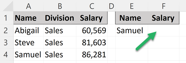
Let’s look up a name and return that person’s salary.

Step 1: Set the starting cell reference

Start writing the OFFSET formula:

=OFFSET(A1,

Step 2: Replace rows argument with MATCH function

The 2nd argument of the OFFSET function determines how much down/up it should return something from. Instead of writing a value here, use the MATCH function to find it automatically.

=OFFSET(A1,MATCH(

Step 3: MATCH lookup value

You use the MATCH function as you normally would. So, start with making a cell reference to the value you want to look for (the lookup value).

=OFFSET(A1,MATCH(E2,

Step 4: MATCH lookup array

The lookup array is the column where you want to search for the lookup value.

When lookup for a name, it’s the “Name” column (column A).

=OFFSET(A1,MATCH(E2,A2:A100,

Step 5: MATCH type

The last argument of the MATCH function determines which type of match you want.

99% of the time, you want an exact match. So, write:

=OFFSET(A1,MATCH(E2,A2:A100,0),

Step 6: OFFSET function columns argument

The MATCH function found the lookup value and knows which row it is located in. It returns that row number to the OFFSET function.

But the last part of the OFFSET function determines which column, in the same row as the lookup value, to return the cell content from.

The “return column” is located 2 columns to the right of the starting cell (the first argument of the OFFSET function, A1).

Your final OFFSET formula should look like this:

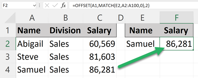
=OFFSET(A1,MATCH(E2,A2:A100,0),2)

And that returns the salary for Samuel. Yay🎉

That’s it – What’s next?

That was how to use the OFFSET function in Excel – aaaaand a whole lot more😉

Like how to make dynamic ranges with OFFSET, how to use OFFSET from the current cell, and how to combine the OFFSET function and the MATCH function.

Although it is very handy – returning ranges with the OFFSET function is a very niche part of Microsoft Excel. It’s not something you need to use all the time.

However, there are other functions you actually do need all the time, like SUMIF, IF, and VLOOKUP.

Please, click here to sign up for my free 30-minute email course that teaches you these functions (and more!).

Other resources

OFFSET is a very unique function that’s almost only useful when combined with other Excel functions.

If you want to take it a step further with niche functions like OFFSET, I suggest you take a look at the INDEX function and INDIRECT function.

Frequently asked questions

Got any specific questions about the OFFSET function?

Read below and you may find your answer😊