How to Lock Columns in Excel (Step-by-Step Tutorial)
Learning how to lock columns in Excel is important for data accuracy and security✅
It means your columns are protected from accidental edits or deletion, especially when you’re sharing your Excel files and working with the team.
In this tutorial, you’ll learn how to lock columns in your worksheet. If you already know how to lock cells, then this tutorial should be familiar and easier to follow. 😎
Download this sample workbook and let’s start!
Step 1: Unlock all cells in the worksheet
When you open our sample workbook, there are specific columns that contain Excel formulas. Aside from formulas, columns might also contain important data and conditional settings we want to maintain.
These are the columns that we need to protect from accidental edits and deletions.
The first step in locking columns in Excel is to unlock all the cells in your worksheet. That is because Microsoft Excel locks all cells by default.
To unlock cells, 👇
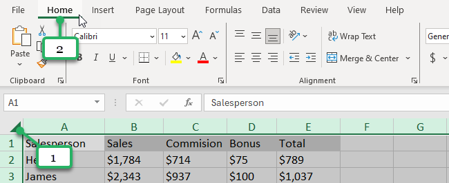
Step 1.1) Select all the cells in the worksheet. You can press Ctrl + A, or click the gray triangle on the top left edge of the worksheet.
Step 1.2) Go to the Home Tab.
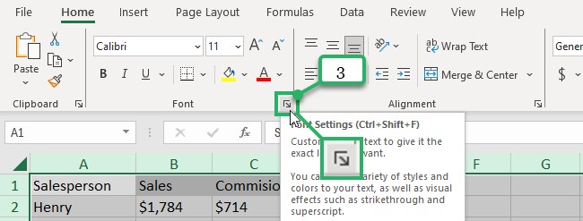
Step 1.3) Click the Format Cells dialog box launcher. This will open the Format Cells dialog box.
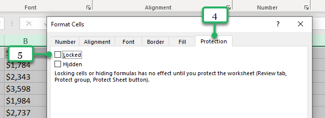
Step 1.4) Click the Protection Tab. You’ll see the Locked and Hidden checkboxes.
Step 1.5) Uncheck the Locked check box.
Step 1.6) Click OK.

Now, all of the cells are unlocked. Let’s proceed. 🔓
Step 2: Lock Specific columns
The next step is to select the columns you want to lock.
In our sample workbook, let’s lock the columns with Excel formulas, column E.
Step 2.1) Select the column header of the column you want to lock. If you want to lock multiple columns at once, press Ctrl and click on other column headers.
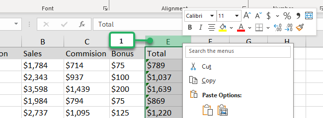
Step 2.2) Right-click on the column header and select Format Cells.

Step 2.3) Click the Protection Tab. You’ll see the Locked and Hidden checkboxes again.
Step 2.4) Check the Locked check box.
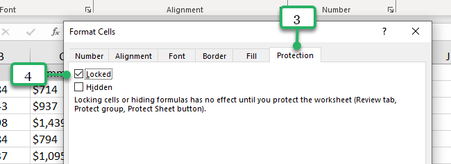
Step 2.5) Click OK.

Take note that doing the steps above has no effect yet on your columns. So, to make this work in full effect, you need to protect the worksheet. 😊
Step 3: Protect Sheet
Step 3.1) Go to the Review Tab.
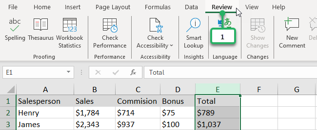
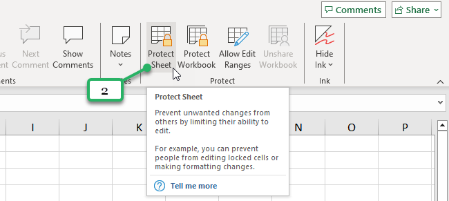
Step 3.2) In the Protect Group, click Protect Sheet. This will open the Protect Sheet dialog box.
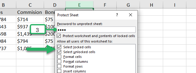
Step 3.3) Create a Password. This will give your worksheet extra protection for anyone who tries to make changes to it. Be sure to create a strong password and remember it, as no one will be able to edit the sheet without entering the password. 🔑
Let’s try to create a simple password for this tutorial like “1234”
Under the “Allow all users of this worksheet to” box, as you can see, two checkboxes are checked by default: Select locked cells and Select unlocked Cells.
There are other actions you can allow users to do in your worksheets such as Format cells, Format columns, and rows, etc.
For now, let’s not make any changes and just check the default ones.
Step 3.4) Click OK.

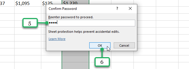
Step 3.5) Reconfirm Password.
Step 3.6) Finally, click OK.
Now this time, you’ve successfully locked columns containing Excel formulas in your Excel sheet. This means all of the cells under this column are locked as well. 🙌
When an Excel user tries to double-click on any of the cells under the locked columns to edit then or move the locked columns, Microsoft Excel sends an error message below.

If another user tries to make any changes to the locked cells, they can click the Unprotect Sheet button in the Review Tab. However, they need to enter the password to unprotect the sheet.
They will need your permission to make any changes to it. 🔐
That’s It—Now What?
Good work! 👏
Learning how to lock columns in Excel means you get to prevent loss of data and protect formulas. You even get to control access and save time when sharing an Excel file with others.
Overall, it gives you peace of mind. 😌
Do you know what else Microsoft Excel can do for you? A whole lot more! You can start learning with these related Excel tutorials below:
