How to Fix the #Name Error in Excel (Step-by-Step)
If you’ve been using Excel for a while now, you must have come across the #NAME error of Excel ⌚
#NAME error is Excel’s way of saying that you’ve made a typo error in your formula. It is a generic error and can occur for any function or formula.
So you need to know everything about this error – starting from the causes to the solutions.
And the guide below will take you through it all 🚀
So stay tuned, and do not forget to download our sample workbook here to tag along with the guide.
Table of Contents
What causes the #name error
The #NAME error primarily occurs whenever you’ve misspelled a name in Excel. Here are some common reasons why the #NAME error might appear in Excel.
Misspelling the name of a function
If you ever get the #NAME error in Excel, go back and recheck the spelling of the function name.
For example, if you type SIM instead of SUM in Excel, here’s what would happen:
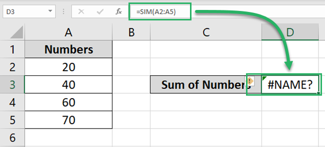
Excel returns the #NAME error because it doesn’t recognize any function by the name SIM.
Misspelled functions make one major reason why the #NAME error occurs in Excel 📌
Misspelling the name of a named range/table
Often when you have named a range or a table in Excel, you’d use the same in your formulas.
Doing so brings ease of reference, but it also brings the risk of getting more #NAME errors in Excel.
Check out below:
This table is named “Numbers” in Excel 🔢
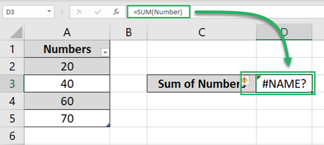
But only because the SUM function has the range misspelled as “Number” instead of “Numbers”, Excel returns the #NAME error.
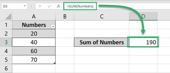
If the same function is run using the correct spelling of the named range, the results would change as below 🎯
Writing the cell range wrong
Often while manually writing the cell range in Excel, users make a mistake.
For example:
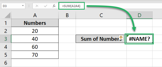
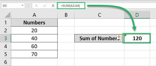
Clearly, we are missing out on a colon sign between the two cell references A2 and A4. And this causes the #NAME error to occur.
Rectify the cell reference from A2A4 to A2:A4 in the formula bar to see the results change as follows 🤩
Writing the arguments wrong
For some functions, you’d need to enter text strings as arguments.
Note that text strings that go as arguments in functions must always be enclosed in double quotes.
If you fail to do so, Excel wouldn’t recognize them as text strings. And you’d have a nasty #NAME error in that cell of your spreadsheet ❔
Check out here:
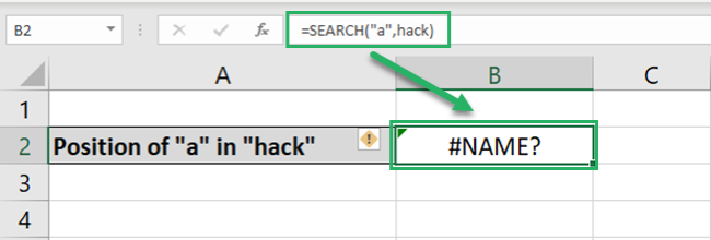
The SEARCH function fails to find the position of the character “a” in the word “hack. That’s because the text string “hack” is not enclosed in double quotation marks.
Let’s enclose it in double quotation marks and reapply the SEARCH function:

The SEARCH function now tells that “a” comes in the second position in the word “hack” 2️⃣
Using an Older Excel Version
Many modern functions are only available in the newer Excel versions (Mainly Excel 2019 and Excel 365).
If you try using these functions in any older version of Excel (where they are not available), you’ll end up with a #NAME error.
For example, try applying the LAMBDA function in Excel 2018, and this is what you get 👵
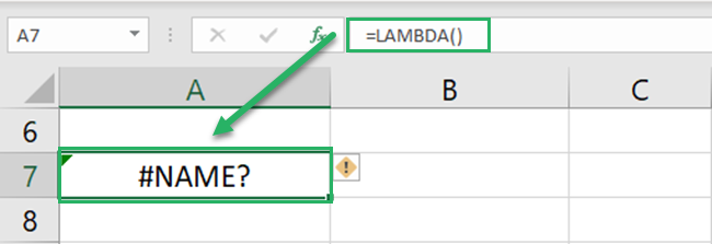
The LAMBDA function is only available to Microsoft 365 users.
The problem remains the same. As the older Excel version doesn’t have this function in its library, it fails to recognize it as a function.
How to fix the #name error
The two biggest reasons that cause the #NAME error – are misspelled function names and misspelled named ranges.
Let’s see how you can fix both of these problems below.
Don’t input functions names manually
Whenever you start writing in a cell with an equal sign, Excel expects you to type a formula (or a function).
And as you start typing the function’s name, say VLOOKUP, a drop-down list of all functions starting with V appears:
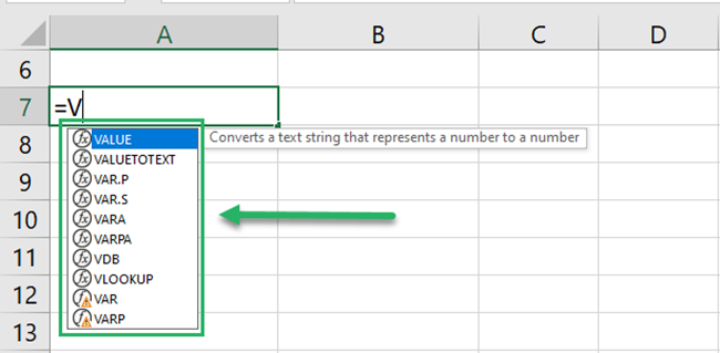
Can’t see VLOOKUP anywhere near the list? Type in the next letter after V i.e. L.
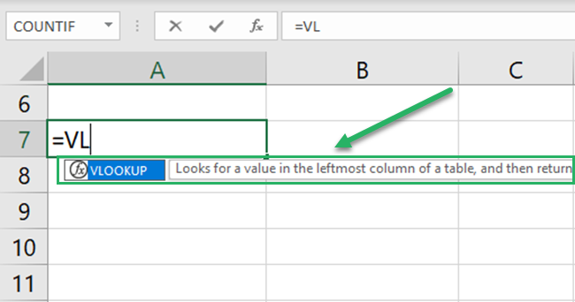
When you’ve found the relevant function, press the “Tab” key.
This enters the complete name of the first function on the drop-down list into the active cell.
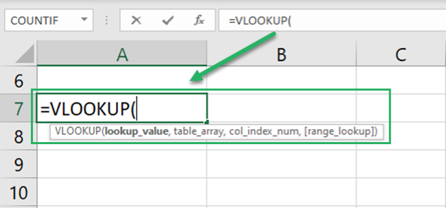
This saves you the chance to misspell the name of the function. And you can safely continue to enter the rest of the arguments.
Pro Tip!
Alternatively, you can also choose the function from Excel’s function library under the Formulas Tab.
Don’t input the names of ranges manually
If you have named a table or a range in Excel, the name will be saved in Excel’s name manager.
For example, here’s a range in Excel.
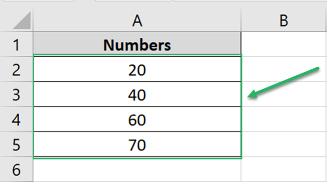
We have named it “Numbers” 🔢

Now, whenever you start writing in a cell with an equal to sign, enter the first letter of this name i.e. “N”.
And Excel will launch a drop-down list of all the named ranges and functions that start with “N”.
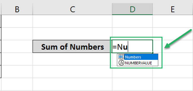
All you need to do is, find the relevant name from this list, scroll down to it and press the “Tab” key.
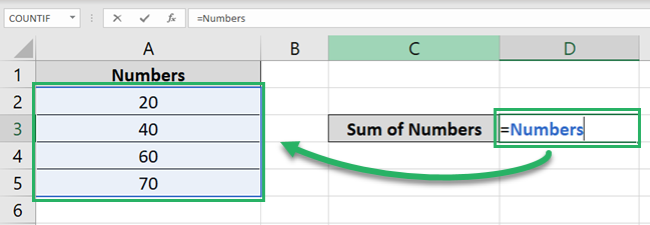
Excel will automatically enter the complete name of the range into your cell.
So there’s no more chance of you misspelling the name of the range.
Pro Tip!
Note that whenever a named range is recognized by Excel, it turns to a color different than black.
Like the word “Numbers” turns blue in the image above 🥶
Examples of formulas that return the #name error
The #NAME error is more of a general error and will occur whenever you misspell a function name.
So you can expect to face the #NAME error in Excel with any function, at any time.
Below, let’s see a few examples of the formulas that return the #NAME error:
Example No. 1: LEFT Function
The LEFT function of Excel extracts the substrings from any given text string.
Let’s extract the first two substrings from the word “spread” using the LEFT function 👈
For that, write the LEFT function as follows:
= LEFT (spread, 2)
The first argument specifies the text string. And the second argument specifies the number of substrings to be extracted from the text string.

Writing it in Excel like that only returns the #NAME error.
That is because the text string in the above function is not enclosed in double quotation marks. And so, Excel fails to recognize it as a text string.
Rewrite the LEFT function as follows:
= LEFT (“spread”, 2)
And see how the results change

Example No. 2: INDEX Function
The INDEX function returns a specific value from a supplied range or table.
However, if misapplied, it might also result in the #NAME error. Let’s see how.
Here we have a table of items in Excel.
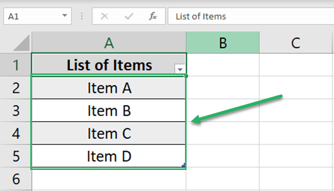
This table is named “ItemsTable” in Excel 💁♀️
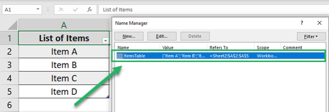
Now let’s write the INDEX function to extract the second item out of this list as below:
=INDEX ( ItemTable, 2 )
This tells Excel to extract the value in the second row of the table.
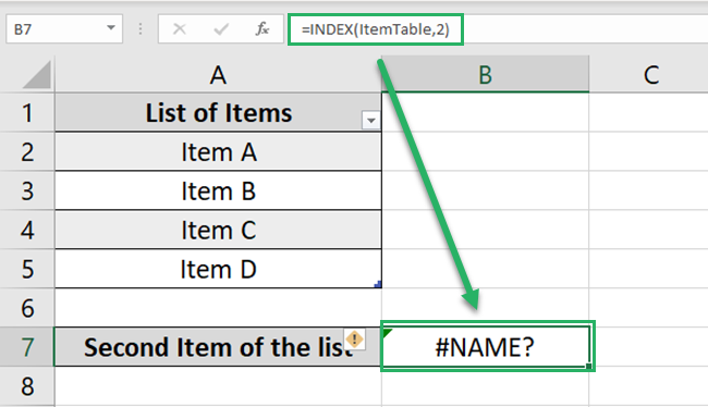
But the function only ends up in an error. Why is that?
We have misspelled the name of the table in the formula above. It’s “ItemsTable” and not “ItemTable”.⚔
Excel fails to recognize the table as its name is misspelled. And so, it returns the #NAME error.
To fix this, rewrite the INDEX function as below:
=INDEX ( ItemsTable, 2 )
This time the results are different.
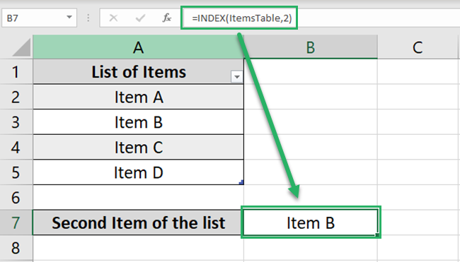
And we have landed on the second item i.e. Item B 🅱
That’s it – Now what
Until now, we have learned what causes the #NAME error in Excel and how can you fix the same.
Additionally, we also came across different examples of formulas that return the #NAME error. You must be feeling like a Pro at Excel now!
If that’s the case, let me tell you – all of these topics make a useful but very small part of Excel. There’s so much more about Excel that you’d want to learn ✨
And at the top of the list come Excel functions. My favorite functions from Excel include the VLOOKUP, SUMIF, and IF functions.
Want to learn them already? Get enrolled in my 30-minute free email course here to learn these (and many more) functions of Excel.
Other resources
Are you trying to run the IFS function in Excel? But every time you do so, you end up with the #NAME error. Hop on here to learn what is causing this error and how may you fix it.
