How to Set Excel Print Titles and Print Headings (2024)

As long as you’re working in Excel, you can freeze the top row and column to scroll to any part of the sheet with them still visible on the sheet 🧐

But very regretfully, the freezing option doesn’t work like that when you print Excel sheets. This means, even if you have frozen panes in Excel, you’ll be able to view the row/column headers on the first print only.

And the rest of the prints will be headerless. If you get to face the same situation, the guide below will teach you how to help it 👇

So download the free sample workbook for this article here and continue reading.

Set row 1 to print on every page (or any other row)

Here’s some data in Excel that extends across many rows.

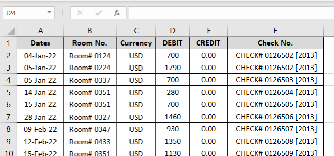
Let me quickly press the Control key + P to preview how it’ll look when printed. The first page looks fine 😎

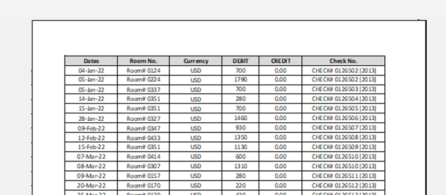
But the second page (and all the pages here onwards) lack the headers on top.

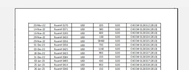
So the data makes only little sense from the second printed page onwards 🙈

Can we not set the print settings such that the headers in the first row (or as many rows) consistently appear on each page when printed?

Sure we can.

1. Go to the Page Layout tab > Print Titles.

You’ll be navigated to the Page Setup dialog box as follows 🚴‍♂️

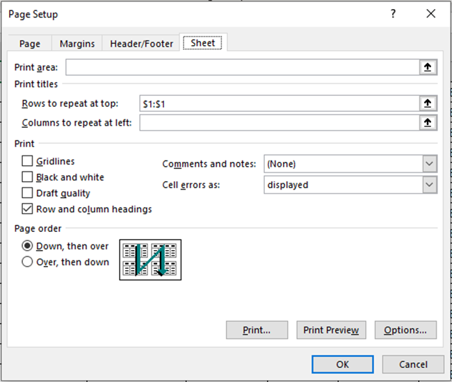
2. Under the Page Setup dialog box, go to the Sheet tab.
3. Lookout for the option Rows to repeat at the top.
4. Click on the collapse button next to it.

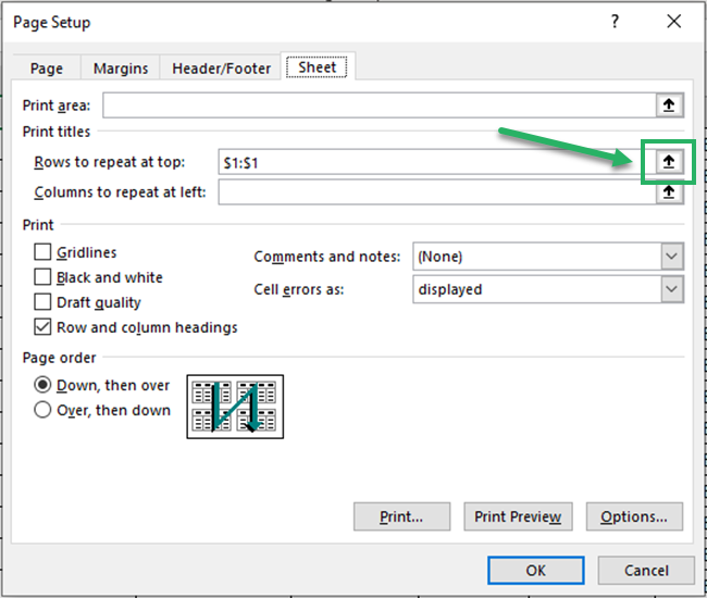
With this, Excel will take you to the worksheet.

5. With the black cursor, select the row headers for the rows that you want to see on each sheet.

We are selecting Row 1 for now 1️⃣

6. Release the cursor once you’re done selecting.
7. Again click on the collapse button.

Excel will take you back to the page setup window dialog box as follows;

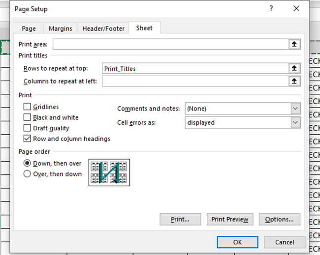
Reference to the relevant rows is created 🔁

8. Click Okay, and that’s it.

Let me now show you the print preview for the second page.

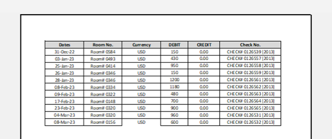
This remains the same for as many pages as are printed 🖨

Pro Tip!

Just like rows, if you want to freeze the first (or any other) column to the left of your prints:

1. Go to the Page Setup dialog box > Sheet tab > Columns to repeat at left.
2. Click on the collapse button next to it.
3. Select the columns that you want to lock on the left.
4. Again click on the collapse button.
5. Click Okay.

How to print headings on each page in Excel

We have seen how you can freeze a particular row or column at the top or left of your sheet in Excel.

However, sometimes, you might want the row headers (1,2,3,..) and the column headers (A, B, C,…) to appear in your prints too 🎧

By default, row and column headers do not appear when Excel sheets are printed. If you want these headers to appear in your prints, this can be done easily.

Repeat Excel header columns and header rows

To see the column and row headers in your prints, follow these steps.

1. Go to the Page Layout tab > Sheet options.

2. Under Headings > check the option for Print 📝

3. Alternatively, you may go to the Page Layout tab > Click Print Titles.
4. Under the Page Setup dialog box > Print > Select Row and Column headings.

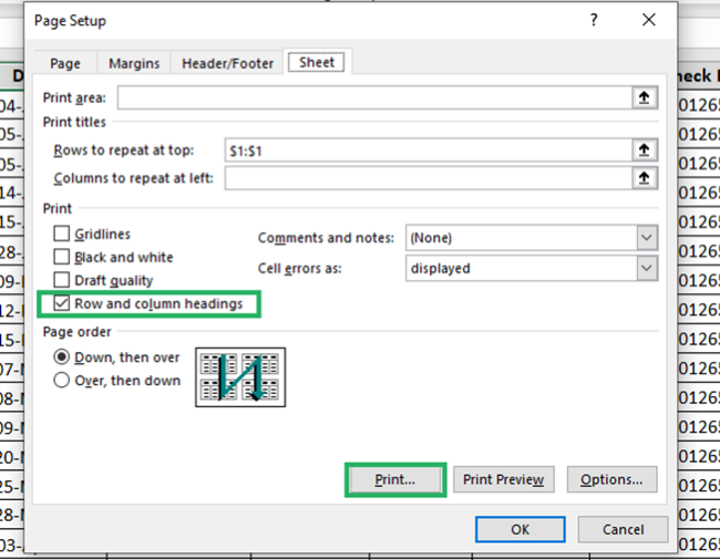
And that’s it – you’re all sorted.

5. Hit the Control key + P to preview the print 🔎

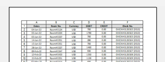
See those headers on the top and the left? It was easy to have them there, wasn’t it?

That’s it – Now what?

Hope you enjoyed learning easy tips on how you can make printing Excel sheets all the more efficient.

However, this is only about printing sheets in Excel. There’s just so much more to Excel that you’re yet to explore 🚀

So let’s get started already? To begin with, I suggest you go with the VLOOKUP, SUMIF, and IF functions of Excel. You’ll be amazed at how useful these functions can be.

Click here and register yourself in my 30-minute free email course right now. It will teach you these functions (and so much more amazing about Excel) in no time.

Other resources

Printing Excel spreadsheets (the way you want them to be printed) is somewhat of a science. But some useful tips can help you master it.

Hop on here to read our blog on how to print labels and gridlines in Excel.