How to Separate Date and Time in Excel (Example)
Excel has a specific format that allows you to populate date and time together in a cell.
Here’s how it looks.
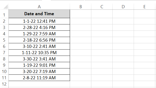
While this is a more comprehensive format, sometimes might not be something you desire. If you have such data at your disposal and you want to separate the columns for data and time, this guide is for you 📝
Managing date and time values effectively in Excel is crucial for accurate data analysis, reporting, and scheduling. There are several techniques that you can use to split data and time values in Excel.
And in this guide, I will walk you through all these methods. So, grab your free practice workbook for this tutorial now and continue reading with me till the end.
Understanding Excel’s Date and Time System
Before we delve into all the methods that come next to split date and time in Excel, we must understand the date and time system of Excel. Particularly, how Excel stores dates and times.
All dates and times are stored in Excel as serial numbers, where 01 January 1900 is 1 and all next dates are numbered as 2, 3, 4, and so on 📆
A date is represented by the integer part of the number (the date value), and the time is represented by the fractional part (timestamp). Hence, a datetime will be a decimal number ⌚
Using Flash Fill and Formulas to Split Dates
The quickest way to separate date and time in Excel is to use the Flash Fill feature.
Flash Fill is a powerful tool in Excel that automatically fills your data when it senses a pattern.
Let me show you how it works to separate data across two columns. To separate the date and time from the list shown above, here’s what we do 📅
Step 1) Activate a cell adjacent to the first row of dates and times.
Step 2) Write in the date only.
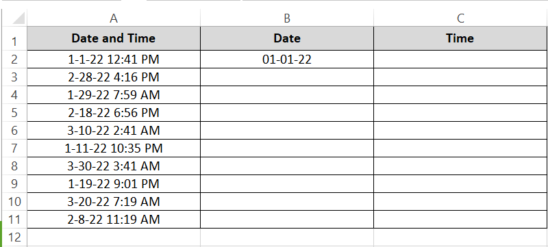
Step 3) Start typing the date in the cell.
By now, Excel should recognize the pattern and suggest the remaining entries for the dates only.
If in any case, Excel doesn’t recognize the pattern for the upcoming entries, select the last cell where you have written the date only and select all the upcoming cells until the last one. Go to the Home tab > Editing group > Fill > Flash Fill. Or, press the Ctrl + E key to trigger Flash Fill.
Step 4) Press Enter to accept the suggestions.
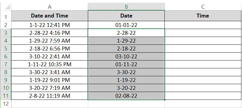
Excel would populate the remaining list of dates only until the last populated adjacent row based on the same pattern as defined above.
Step 5) Repeat all the steps above for a separate column of times.
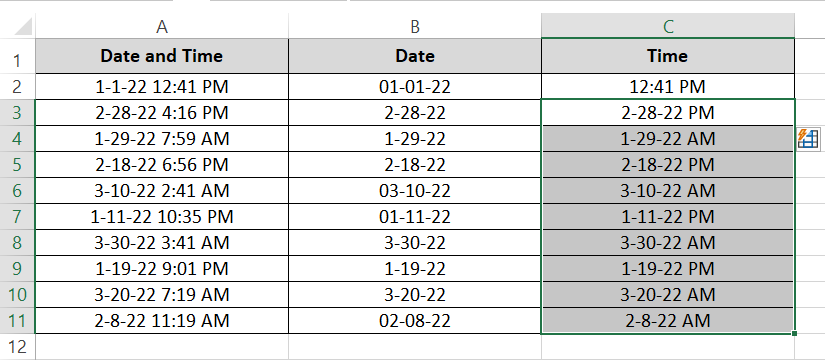
Flash fill makes the job easy and quick.
The Flash fill feature is not dynamic. If you make any changes to the original list of dates and times, this column for the dates will not automatically change.
Using the INT and MOD Function
The INT and MOD function make a dynamical way to extract date and times from a cell in Excel. Check this out 🚀
Step 1) Activate the cell where you want to extract the date.
Step 2) Write the INT function in it as follows:
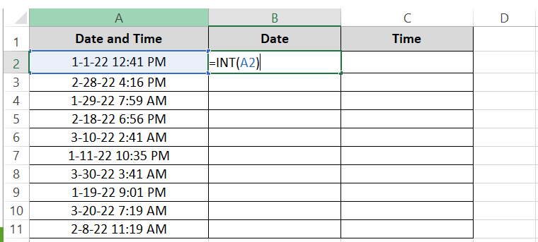
The INT function extracts the Integer from a given number (leaving out the decimal points). Excel stores dates as integers and time as the decimal number so if you eradicate the decimal number leaving behind the integer, technically you’ll get the date only (without time).
Step 3) Press the Enter key.
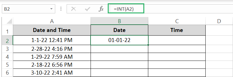
Step 4) Drag this function down the list of all dates and times to extract the dates only.
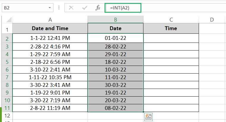
Step 5) Activate a cell from a new column.
Step 6) Write the MOD function in it as follows:
The MOD function of Excel returns the remainder after a number (dividend) is divided by another number (divisor). So, if you extract only the decimal portion of a number (leaving out the integer), you will get the times extracted only.
Step 7) Press the Enter key.

Step 8) Drag this function down the list of all dates and times to extract the times only.
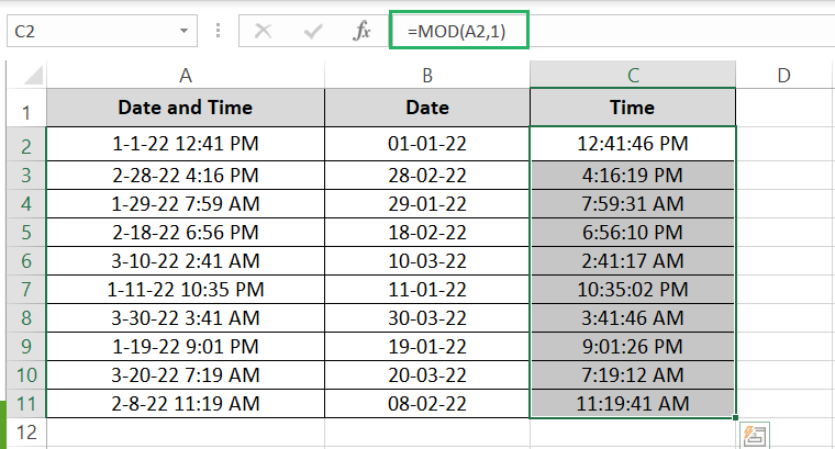
Good to go! This is another easy way to separate dates and times. Make sure to format the separated columns as Short Date and Time.
The plus point is that this is a dynamic way to separate dates and times. As you make any change to the original list of dates and times, the separated dates and times will automatically change 🧪
Using Text to Columns Feature
The Text to Column feature is a data-splitting tool of Excel. You can also use it to separate dates and times in Excel.
Step 1) Select the cells containing dates and times.
Step 2) Go to the Data tab > Data Tools > Text to Columns.

Step 3) From the Text to Columns Wizard, select Fixed Width.

Step 4) Click Next.
Step 5) Drag the scale between the dates and times.
Step 6) Mention the destination cell where you want the split columns to be placed.
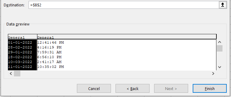
Step 7) Click on the Finish button.
The dates and times will be split between two columns.
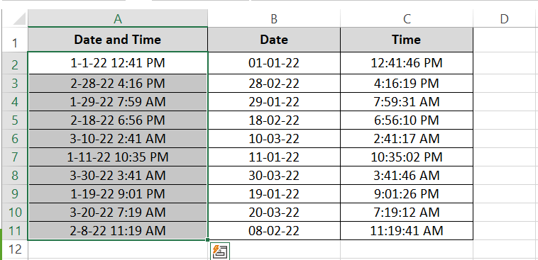
The date and times column will be split into two columns ✂
Extract the Date and Time using the LEFT and RIGHT functions
The LEFT and RIGHT functions in Excel are used to extract a specified number of characters from the beginning or end of a text string, respectively.
The LEFT function extracts text strings from the left of a text string and the RIGHT function extracts the text strings from the right of a text string 😎
Here’s how you can use it to separate dates and times in Excel.
Step 1) Write the LEFT function as follows;
Step 2) As the first argument, refer to the cell containing the date and time value.
Step 3) For the next argument, nest in the FIND function.

Since we want to extract the integer portion of the number in Cell A2 only (that represents the date), I have written the FIND function to return the position of the decimal point “.” from Cell A2.
Then deduct 1 from this position because we want to extract the numbers before the decimal point only. And nest this in place of the num_chars argument of the LEFT function that tells it the number of strings to extract from the left of the text string in Cell A2.
Step 4) Press Enter.
Excel will extract the integer portion from Cell A2.
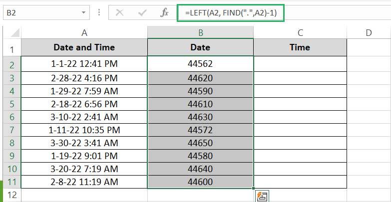
Using the same science, we will extract the time from Cell A2.
Step 5) Write the RIGHT function as follows;
Step 6) As the first argument, refer to the cell containing the date and time value.
Step 7) For the next argument, nest in the LEN and FIND function.

This time, we want to extract the decimal portion of the number in Cell A2 only (that represents the time), I have written the FIND function to return the position of the decimal point “.” from Cell A2.
And then deducted it from the total length of the strings in Cell A2 (the LEN function returns the length of the text string in a given cell) 🙌
Add a 1 to it so we have the decimal numbers + the decimal point for Excel to recognize it as a time.
This makes it 9 less 6 plus 1 = 3. So, the RIGHT function will extract the last three characters from Cell A2.
Step 8) Press Enter.
Excel extracts the decimal portion of Cell A2.
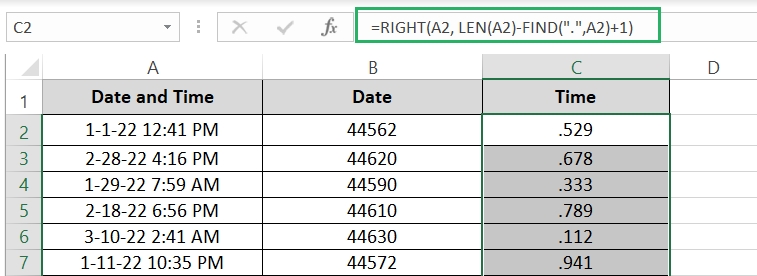
Step 9) Copy both these columns by pressing the Ctrl + C key.
Step 10) Paste them as values by pressing the Alt key > E > S > V.
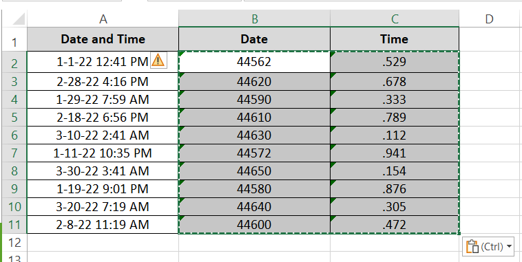
If you see the Error triangle next to any pasted value, select all such cells, right-click on them, and from the drop-down menu, click on Convert to Number.

Here’s how it looks post conversion.

Step 11) Select the column of dates (the integers).
Step 12) Press the Ctrl key + 1 to launch the Format Cells dialog box.
Step 13) Set the Number format to Short Date.
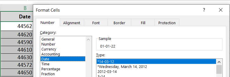
Step 14) Select the column of times (the decimal values).
Step 15) Press the Ctrl key + 1 to launch the Format Cells dialog box.
Step 16) Set the Number format to Time.

By now, you’d have both the dates and time columns separated with proper formatting.
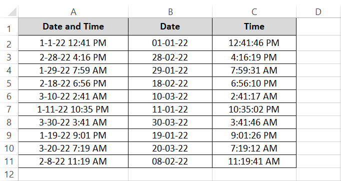
I find this is a relatively longer method so this one’s not very preferable for me.
Separate Date and Time in Excel by changing the Number Format
This method is not a very robust one, this is only for visual representation purposes.
If you are not concerned with what goes behind the cell but only want to split the dates and times on the face of the sheet, try doing this 👇
Step 1) Make two copies of the original column of dates and times.
Step 2) Select one of these column copies.
Step 3) Press the Ctrl key + 1 to launch the Format Cells dialog box.
Step 4) Set the Number format to Short Date.

The column will only show dates since the format is set to short date. However, when you go to the formula bar, you will still see the complete date and time running behind the cell.
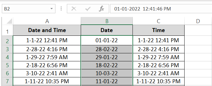
Step 5) Select the other copy of the column.
Step 6) Press the Ctrl key + 1 to launch the Format Cells dialog box.
Step 7) Set the Number format to Time.
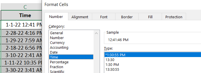
The column will only show times since the format is set to Short Time. In the formula bar, however, you will see both the date and time behind the cell.
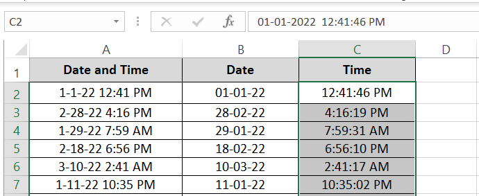
This is also a way how you can split dates and times into two columns in Excel.
Set up a Power Query
The Power Query method to split date and time in Excel is a little longer and may be more complex than the previous methods ⚒
However, if you have such data at your disposal frequently, you can save this query and re-run it again and again to save time.
So, let’s try it out and see how you can split date and time in Excel by using the Power Query editor.
Step 1) Select the data range containing the names.
Step 2) Go to the Data tab > Get & Transform Data > From Table/Range.

This will launch the Power Query Editor with the selected data loaded into it as below.
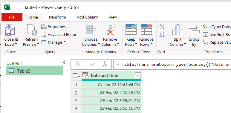
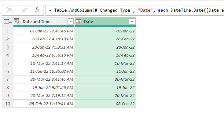
Step 3) Within the Power Query Editor > Go to the Add Column tab > From Date & Time group > Date > Date Only.

The Power Query Editor will add a new column containing the dates only.
Step 4) Select Column 1 again.
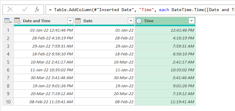
Step 5) Within the Power Query Editor > Go to the Add Column tab > From Date & Time group > Time > Time Only.

The Power Query Editor will add a new column containing the times only.
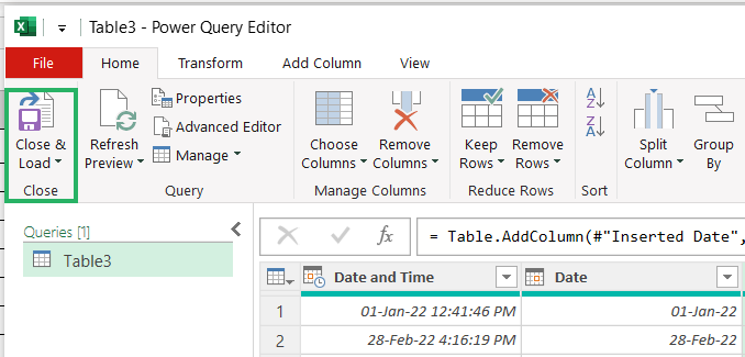
Step 6) Click on the Close & Load button on the top right of the Power Query Editor.
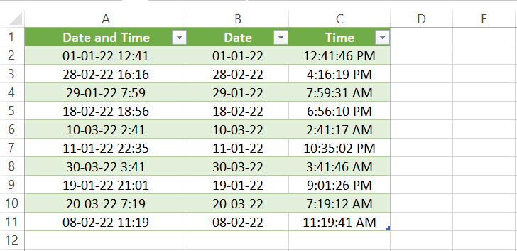
You’ll see three columns added to a new worksheet of your workbook. The original dates and times, a separate column for dates, and a separate column for times 🔎
It is not advisable to use this method if you’re only looking to split date and time in Excel. However, if this is something that you get to do often, setting up a Power Query for it can help you job in big time.
Conclusion
In this guide, we have seen a variety of methods to separate dates and times in Microsoft Excel. Starting from the easiest Flash Fill method to using multiple functions like INT, MOD, LEFT, and RIGHT functions.
And not only that but also advanced tools like Text to Columns and Power Query Editor. Try out these methods to see which one suits you the best.
Before you move on, read the following Spreadsheet Excel tips and Excel tutorials on similar topics.
