How to Do VLOOKUP in Excel with Two Spreadsheets (Easy)

Dealing with a dataset too big that’s spread across more than one sheet? And now you want to dynamically look up this data to find values?

This tutorial has you sorted 🥤

Just like we use VLOOKUP to look at values within a sheet, you can use it to look at data with two spreadsheets, too. And believe me, it’s easier than you think.

To see how it works step-by-step, download the free practice workbook for this tutorial here and read with me till the end.

Table of Contents

VLOOKUP in Excel

The VLOOKUP function is undoubtedly the most common function of Excel. It is used to look up data vertically.

It finds data from a column based on a given value that is located in another column.

Syntax

For some quick revision, here is what the VLOOKUP function’s syntax looks like 👀

Where:

• Lookup_value is the value to be looked up for. It must be situated in the leftmost column of the table_array.
• Table_array is the cell range where the lookup_value is located and from where the resulting value is to be returned.
• Column_index_number is the column number from where the values are to be returned.
• Range_lookup is an optional argument that defaults to TRUE or 1 (approximate match). To get an exact match, set it to FALSE or 0.

Basic Example

Before I show you how VLOOKUP works with two spreadsheets, let’s quickly brainstorm how it works within a single sheet (very simple and basic).

Here is a dataset of some student’s marks and ages entered in Excel 📈

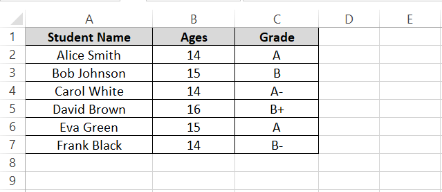
Close your eyes and imagine this list is not only 6 rows but thousands of rows long 😜

And out of this very huge data we need to find the grade of a student, say Alice Smith.

Here’s how you’ll set up the VLOOKUP function to fetch the grade of Alice Smith from this dataset.

Step 1) Begin with writing an equal to sign and then the VLOOKUP function.

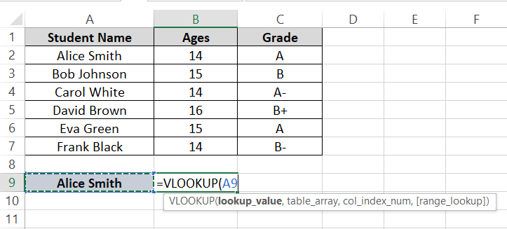
Step 2) As the lookup value, refer to the cell that contains the student name whose grade is sought.

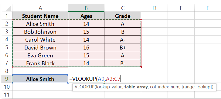
Step 3) Define the table array starting from the column that contains the student names.

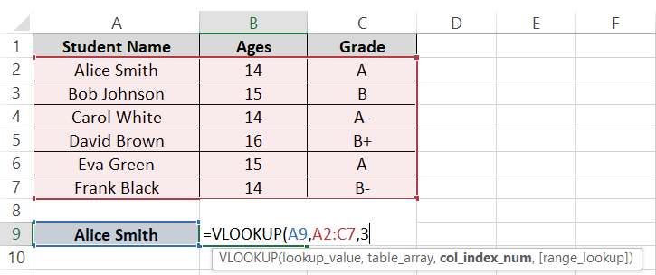
Step 4) As the column index number, write 3. This is because grades (that we want Excel to return) are populated in the third column starting from Column A (the first column of the table array).

Step 5) For the range lookup mode, define FALSE as we want Excel to return the exact match.

Step 6) Press Enter 🔑

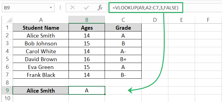
There it is. VLOOKUP fetches the grade for Alice Smith from the data that’s A.

This is how basic VLOOKUP works in Excel. Guess we’re done revising the basics. Let’s now move to the next section that explains how you can VLOOKUP data between two sheets.

Doing VLOOKUP in Excel with Two Spreadsheets

Doing VLOOKUP in with two Excel sheets (actually multiple sheets) is not very different from doing VLOOKUP in a single sheet 🚀

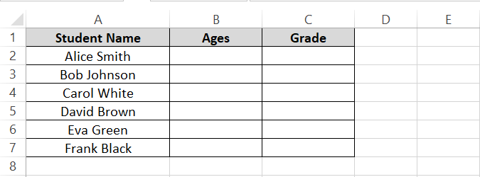
Going with the same data as above, the only difference is that this time we want to fetch the age and grade for these students.

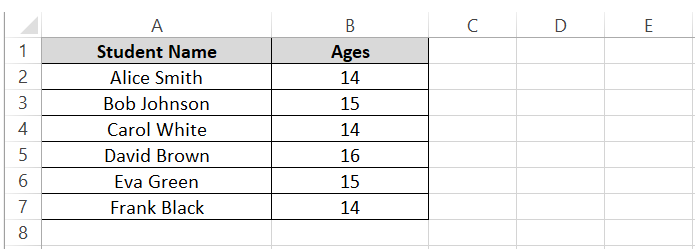
However, the ages are populated in another sheet.

Surprisingly, the grades are also populated in altogether another sheet.

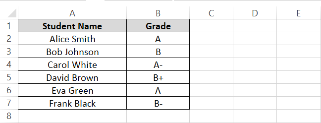
However, we have student names present in all sheets, so taking it as the common data point, fetching all this data together in one sheet shouldn’t be a problem 📝

Let’s begin the looking up the dataset to find the ages of students.

Step 1) Write the VLOOKUP function as follows.

Step 2) As the lookup value, refer to the cell containing the student’s name.

Step 3) To define the table array, go to the sheet that contains students’ ages.

Step 4) Select the range of cells containing this data. Excel will pick the sheet and cell reference automatically.

Pro Tip!

It is advisable to go to the other sheet and select the cell range as the table array to let Excel do the referencing job (easy and error-free).

But you can also hardcode the sheet reference into the VLOOKUP formula. It’s simple. Write it as 👇

SheetName!CellReference

Write the sheet name, add an exclamation mark, and then the cell range reference. This sheet is named “Ages”, so the table array reference becomes:

Ages!A2:A7

Same as Excel referenced it automatically in the above formula.

However, if the sheet name contains any space characters or non-alphabetical characters, then you must enclose it in single quotation marks. For example, if the sheet name had been “Ages of students”, the above table array reference would have been written as:

‘Ages of students’!A2:A7

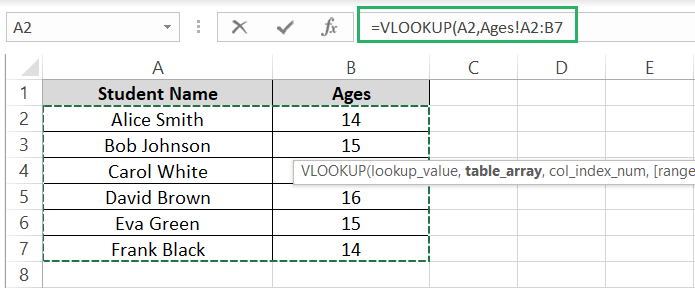
Step 5) Stay on the same sheet.

Step 6) Define the col_index_number as 2 as the ages of students are populated in the second column of this table array.

Step 7) Set the range lookup mode to FALSE.

Step 8) Close the parenthesis.

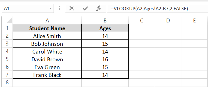
Step 9) Now press Enter.

Excel will navigate you back to the original sheet where you started typing the formula and the results will fascinate you 😲

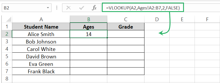
VLOOKUP from another sheet returns the correct age for Alice Smith.

Step 10) Change the table array reference to absolute by activating the formula, going to the table array reference, and pressing the F4 key.

This is so that the table array reference doesn’t change as we drag and drop this formula down.

Step 11) Drag and drop it down to have the ages look up for all the students.

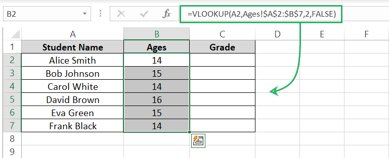
And voila! VLOOKUP returns ages for all the students from another Excel sheet in a single go.

Let’s now fetch the grades of students from the sheet for grades 🚴‍♀️

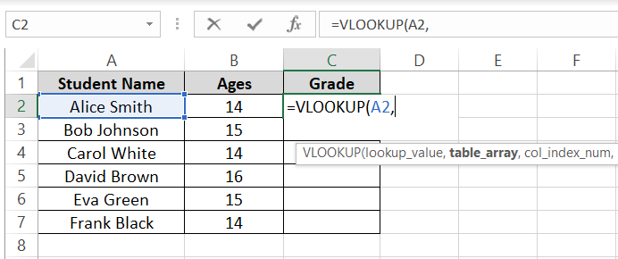
Step 1) Activate the relevant cell in the sheet where you want the grades fetched.

Step 2) Begin writing the VLOOKUP function as follows.

Step 3) As the lookup value, refer to the cell containing the student’s name.

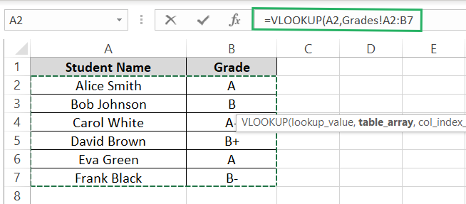
Step 4) To define the table array, go to the sheet that contains students’ grades.

Step 5) Select the cell range containing this data and let Excel pick the sheet and cell reference automatically.

Alternatively, you can hardcode it yourself as Grades!A2:A7.

Step 6) Stay on the same sheet.

Step 7) Define the col_index_number as 2 as grades of students are populated in the second column of this table array.

Step 8) Set the range lookup mode to FALSE.

Step 9) Close the parenthesis to conclude the VLOOKUP formula.

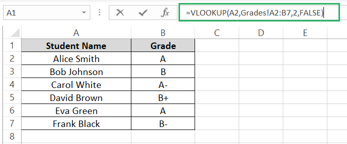
Step 10) Now press Enter.

Excel finds you the grade for Alice Smith from another sheet. Wow!

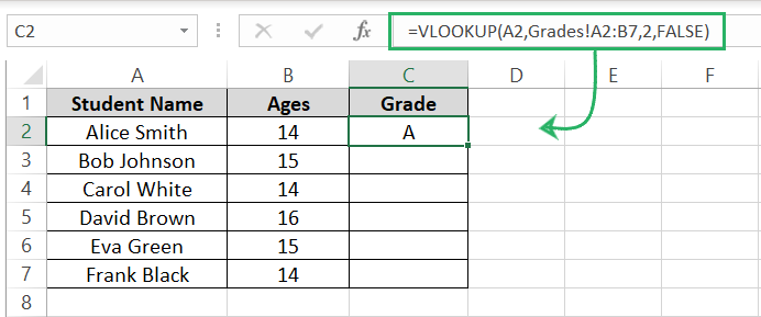
This is great. To populate the whole row for grades of students:

Step 11) Activate the formula.

Step 12) Go to the table array reference and press the F4 key to convert the table array reference into an absolute reference.

Step 13) Drag and drop this formula down to have the grades for all students looked up from the sheet for Grades.

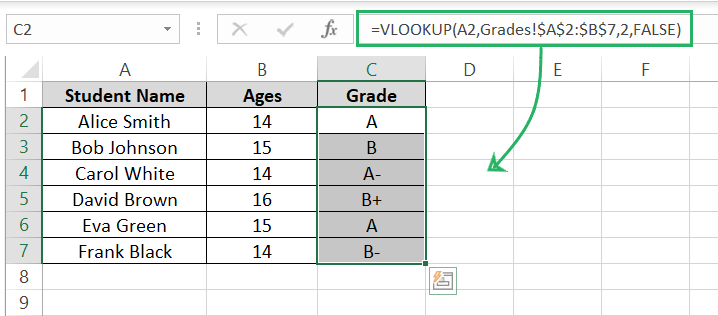
There you get it! VLOOKUP function fetched the ages and grades of all students from two different spreadsheets.

This shows how easy it is to use VLOOKUP across more than one sheet. As you’ve seen, it’s as simple as a basic VLOOKUP ✌

Conclusion

After you’ve read this guide, you can now do VLOOKUP with two spreadsheets of Excel. So even if you’re working with dense sets of data that are spread across multiple spreadsheets, you know how to fetch it in place.

Frankly, this tutorial is an example of how Microsoft Excel allows you to dynamically store and sort data. VLOOKUP is the heart of Excel, and this tutorial only explains one way of making the most out of VLOOKUP’s potential 🙈

Learn more about it through the following Spreadsheeto tutorials.

• How to Use VLOOKUP in Excel: 4 Easy Steps (For Beginners)
• VLOOKUP Not Working? Here Are 5 Methods to Fix it
• VLOOKUP with Wildcards in Excel (2024 Guide)