VLOOKUP Not Working? Here Are 5 Methods to Fix it
VLOOKUP is the universal lookup function that everyone’s heard about 🔊
But it might be a little tricky to operate it at times. Especially when it starts throwing errors your way.
Is your VLOOKUP also not working? In the guide below, we have collated 5 main reasons why this might happen along with the methods to fix them.
Download the sample workbook for this guide here and dive in straight 📩
Table of Contents
Values stored as text
One of the most common reasons you can expect VLOOKUP to malfunction is the wrong formatting of the values.
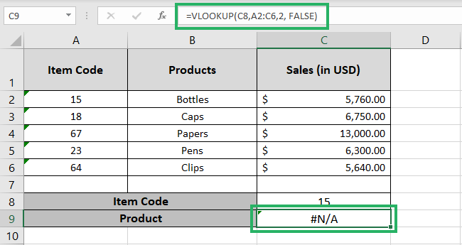
For example, in the image below, we have some items along with their item codes 👀
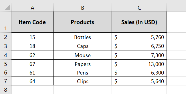
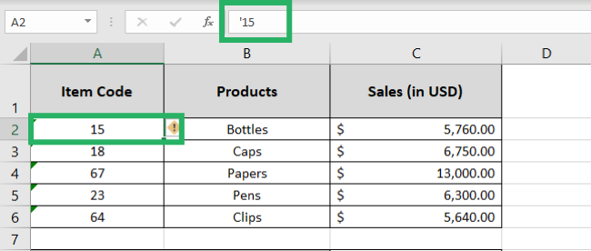
These product codes are stored as text. This may be because of the formatting applied to them. Or if they have an apostrophe before them like here.
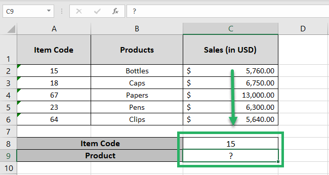
Now let’s say we want to find the product against Product Code 15 here.
If we apply the VLOOKUP formula as follows:
=VLOOKUP(C8,A2:C6,2,FALSE)
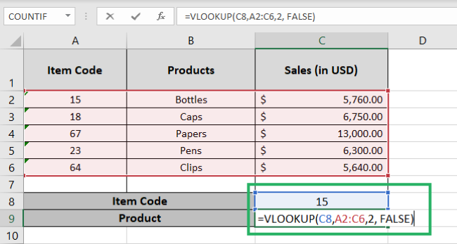
And this is what you get. The #N/A error.
But if we change the format of the Product codes in the lookup range and convert them into numbers, the results would be different.
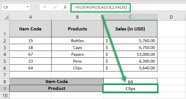
So if you are having a tough time figuring out the reason for the #N/A errors your VLOOKUP has been posing, double-check the format of the values you’re using 📝
An easy way to change the format from Text to Numbers is by clicking on the cell. And then click on the error icon that comes next to it.
From the menu of options, select ‘Convert to Numbers’ 🔢
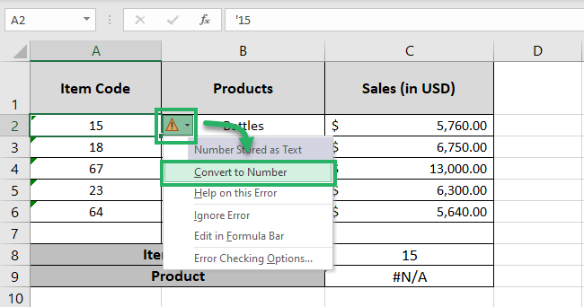
Forgot the exact match argument
The VLOOKUP function has four arguments. The last argument is the range_lookup argument which is an optional one.
This argument specifies if an exact or approximate search is to be performed 😵
Pro Tip!
Under the exact mode, the VLOOKUP function looks for the exact lookup value. And if it is not present in the dataset, VLOOKUP returns the #N/A error.
However, under the approximate match mode, the VLOOKUP function looks for the exact lookup value or the next smallest value. However, for the approximate match mode to run correctly, the data must be arranged in ascending order 🏹
To perform a search under the exact match mode, the fourth argument must be set to FALSE. If left omitted, Excel sets it to the approximate match mode (TRUE) by default.
Now how does this cause the VLOOKUP to malfunction? See here:
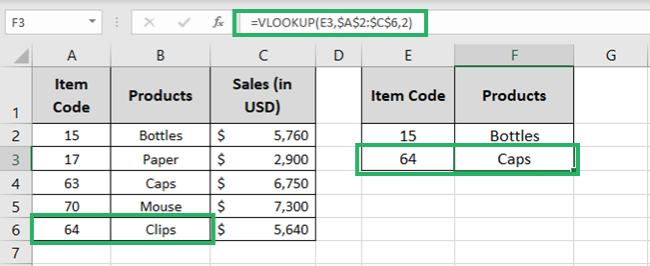
For Item Code 64, the VLOOKUP function returns the product ‘Caps’. However, that’s not the correct answer. We can see the product against Item Code 64 is ‘Clips’ ❌
This happened because we forgot to write the range_lookup argument in our VLOOKUP function. So it was set to an approximate match mode (TRUE) by default.
The approximate match mode needs the data arranged in an ascending order which was not the case in our example. The Item Code at Row 4 is 70 (greater than the lookup value of 64). That’s where Excel stopped searching and returned the Product against the Item Code equal to or next smallest to 64 🤷♀️
From the numbers 15, 17, and 63, the next smallest to 64 is 63 and so we get the product against the Item Code 63 i.e. ‘Caps’.
Now let’s rewrite the same function with the exact match mode as follows:
= VLOOKUP (E3, $A$2:$C$6, 2, FALSE)
The results this time will be different (and correct):
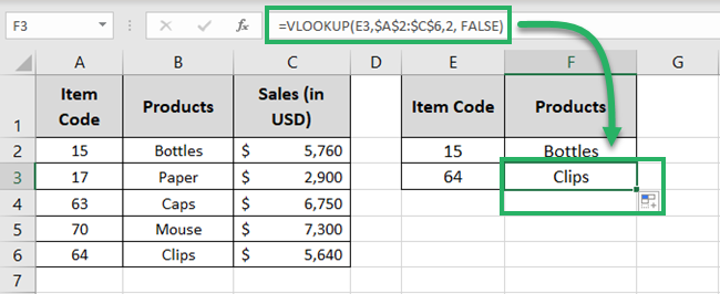
This time Excel doesn’t stop searching at 70.
If you’re looking for an exact match, do not forget the exact match mode argument 🔎
Unlocked cell references
You might not even notice this – but this is a big, big problem when using VLOOKUP.
Let me explain this through an example. The example we’re using is the same as above (Item codes and products).
However, here is a list of Item codes for which we need to find the Product from the lookup range 🧐
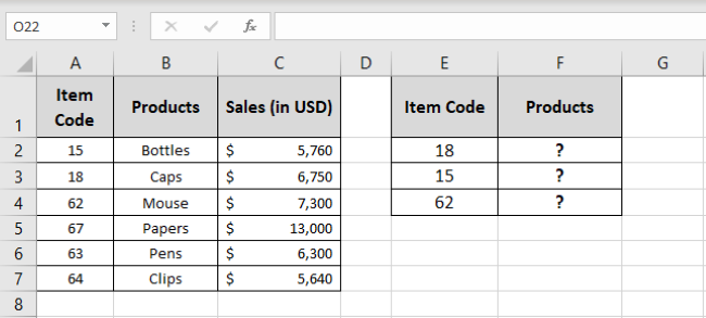
- To do that, let’s write the VLOOKUP function below.
= VLOOKUP ( E2, A2:C7, 2, FALSE)
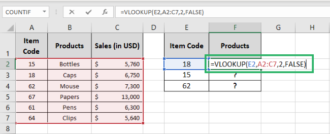
We have referred to E2 as the lookup value, cell range A2:C7 as the lookup range, and 2 as our column number from where we want the value (it is the column of Product names).
Note the relative references we used for the lookup range i.e. A2:C7.
- Hit Enter to get the results.
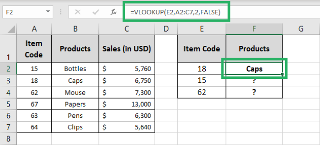
Everything seems good until now.
- But drag and drop the same formula to the remaining list, and this is what happens.
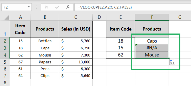
Instead of the product names, we get the #N/A error. That’s because we dragged and dropped the formula. Excel updated the lookup value from E2 to E3.
But at the same time, it also updated the lookup range from A2:C7 to A2:C8.
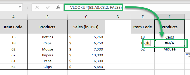
As the lookup range has changed, Excel fails to find the subject lookup value and you get the #N/A error.
This happens when the cell references for the lookup range are left unlocked with the VLOOKUP function.
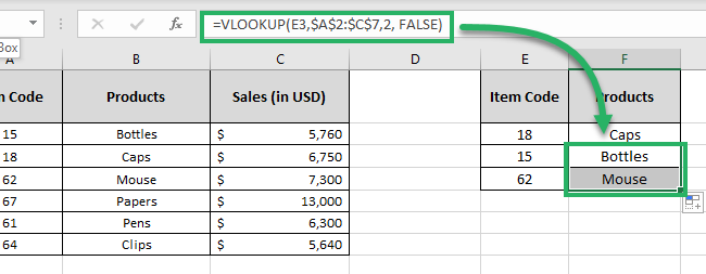
To help this problem, you must always turn the lookup range in your VLOOKUP formula to an absolute reference.
To change a cell reference from relative to absolute, go to the formula bar, click on each cell reference, and press the F4 key.
So after we have changed the formula above to this:
= VLOOKUP (E2, $A$2:$C$7, 2, FALSE)
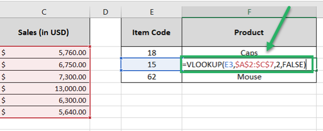
The results change as follows:
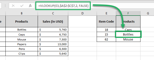
No more #N/A errors! This time Excel only updated the cell reference for the lookup value. Whereas the lookup range remains the same.
Inserted columns in the lookup table
The VLOOKUP function requires a col_index number to return the desired value, remember?
For example, in the image below, we defined the table range as A2:C7 and the column index number as 2.
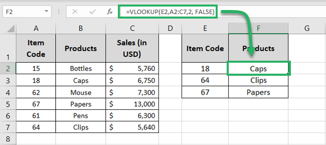
So Excel returned the corresponding value from column 2 of the defined range i.e. Column B (Products).
Now try adding a new column to this table before column B. And the results would go crazy, as shown below 🥴
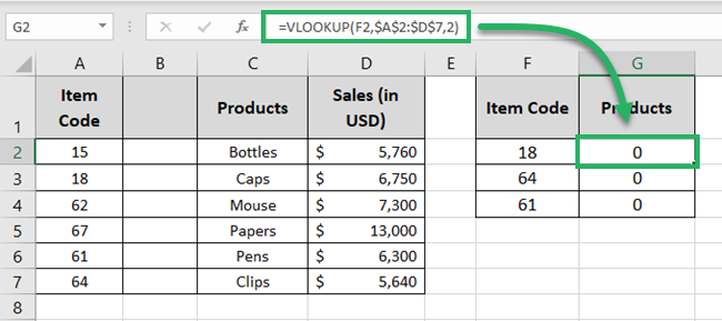
The result changed to 0. This is because as you added a new column, Excel updated the table range from A2:C7 to A2:D7. And column number 2 from this range is again Column B which is now vacant.
So Excel returns 0.
How can you help this situation? Use the MATCH function instead 🪁
Instead of manually supplying a static column index number, let the MATCH function do that.
Write the MATCH function to find the column number like below.
= MATCH ($F$1, $A$1:$C$1, 0)
It will return the column number of the lookup value i.e. F1 (Products) from the headers of the lookup range 🙈
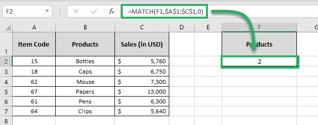
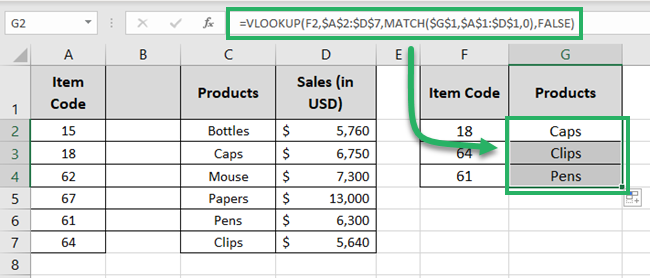
So even if you add a column, the MATCH function will automatically update the column number.
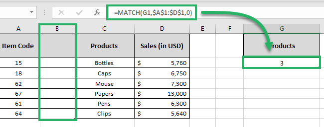
The VLOOKUP function will change as follows:
= VLOOKUP ( E3, $A$2:$C$7, MATCH ($F$1, $A$1:$C$1, 0), FALSE)
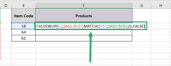
Now hit enter and add or delete any column, the results won’t change.
New data in the table not included
If you add new rows to your data, don’t expect the VLOOKUP function to identify them and include them in the lookup range automatically.
The image below shows the VLOOKUP function applied 👇
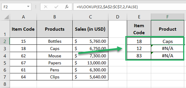
You’d see there are a few item codes in the second table that are not present in the first table. And so, the VLOOKUP function returns the #N/A error for them.
Now if we add a few more rows to the lookup range as follows:
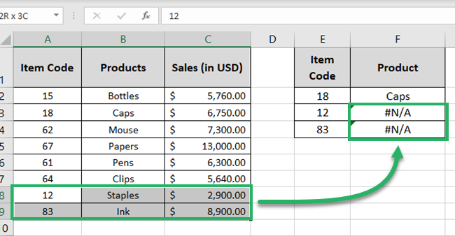
Nothing changes 🚩
That’s because the lookup range for the VLOOKUP function has not changed. Excel hasn’t updated the lookup range for the new rows added.
How to help with this problem?
You can convert the lookup range into a table. To do this, select the range (A1:C7), and go to the Insert Tab > Table.
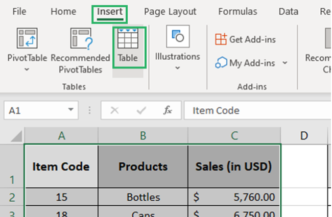
Once the lookup range is converted into a table, whenever you add a new row just beneath the table, Excel makes it a part of the table.
And as the lookup range now refers to the table and not any specific cells, it is automatically updated for any new data additions 🚴♂️
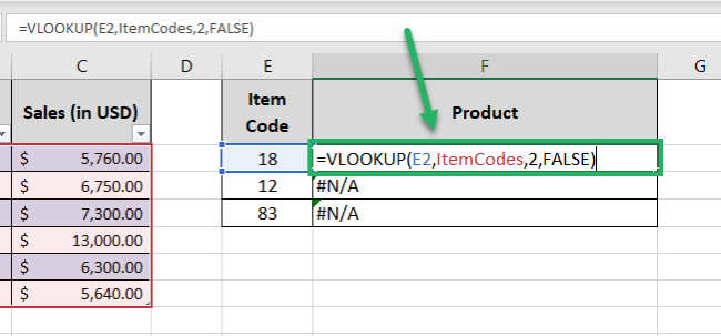
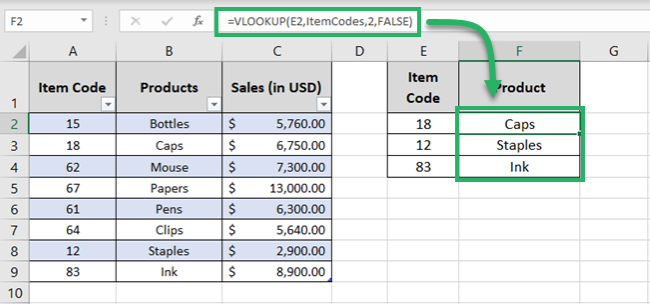
We have named our table as ItemCodes 📜
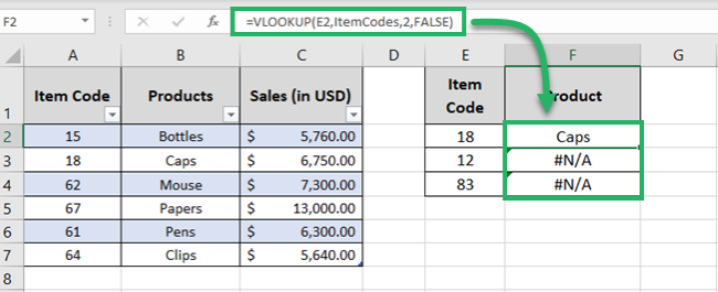
Now whatever you add to the table will be automatically updated in the VLOOKUP formula. So, the results change as follows:
You are searching for nonunique values
If you are not getting the expected results from your VLOOKUP function but something different, maybe you are searching for non-unique values.
For instance, the data below has duplicate item codes (Code 15 occurs twice) 2️⃣
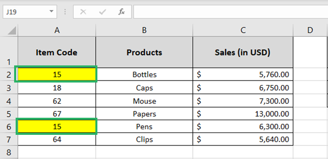
Now let’s write the VLOOKUP function to find the product against Item Code 15.
= VLOOKUP (E2, A2:C7, 2)
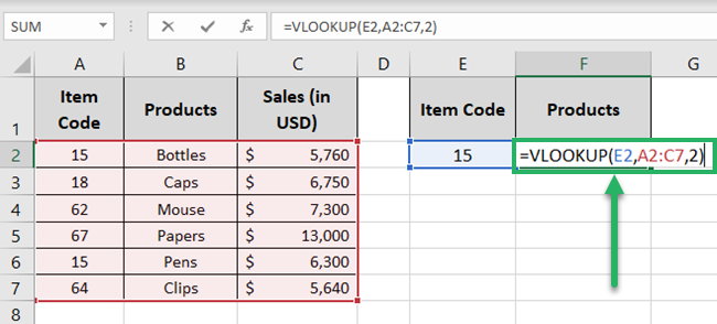
Hit Enter to see what happens.
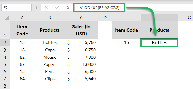
The VLOOKUP function returns the product ‘Bottles’ 🍾
Although we had two products against Item Code 15 i.e. Bottles and Pens. But the VLOOKUP function only returns the first instance (Bottles come first when seen top to bottom).
So if your data has duplicate values, the VLOOKUP will return the results for the lookup value 🥇
To help this situation, you must delete any duplicate values from your data first. This can be done using the Remove Duplicates tool of Excel.
To use the Remove Duplicates tool:
Select the data and go to the Data tab > Data Tools > Remove Duplicates.
That’s it – Now what?
Try using the methods above to sort the problems VLOOKUP has been tossing your way. And you’d get through it.
Don’t stop just there. These were only 5 main problems of the VLOOKUP function. Excel has a whole library of functions, features, and tools for you to uncover 🎯
Start by learning more about the VLOOKUP function, SUMIF, and the IF functions. How to do that? Click here to enroll in my 30-minute free email course that is designed to teach you these (and many more) Excel functions.
Happy spread-sheeting to you!
Other resources
The VLOOKUP function can be of great help when used the right way.
