VLOOKUP with Wildcards in Excel (2024 Guide)

The VLOOKUP function is one of the most used and powerful Excel functions 💪

It helps us look up values from our datasets in a few seconds.

What makes the VLOOKUP more powerful is that you can find lookup values from partial matches too 🤯

That’s possible by using wildcards in your VLOOKUP formulas.

In this lesson, you’ll learn exactly how to use VLOOKUP with wildcards in Excel 😀

Learn and practice in real-time by downloading this free Excel worksheet linked.

Types of wildcards to use with VLOOKUP

In Excel, wildcard characters are used to do partial matches *️⃣❔

Excel supports three different kinds of wildcard characters.

• Asterisk – *
• Question mark – ?
• Tilde – ~

All three of these wildcard character types are acceptable in a VLOOKUP function.

An asterisk wildcard character is used to represent any number of characters when doing a partial match.

For Example, Sp* could match Spreadsheeto, Special, Space, etc.

Question mark wild character represents any unknown single character.

For example, P?n will match Pan or Pen or Pin 🍳🖊️📍

The tilde wildcard character helps to remove the effect of other wildcard characters.

For Example, if you have to search exact match for “Excel*”, you have to enter “Excel~*”. Otherwise, you will get all words beginning with the word “Excel”.

You can learn how to use wildcards in VLOOKUP using the below Examples.

VLOOKUP wildcard formula example #1: Asterisks as wildcards

The below data set shows the quantity for each shoe type in a shoe shop 👞👟

Assume that you want to find the quantity of Derby shoes from the above table. But, note that you have entered only “Derby” in the lookup value.

Then, you can follow the below steps.

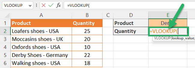
1. Enter an equal sign and select the VLOOKUP function.

Then, your formula bar will show;

=VLOOKUP(

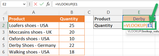
2. Select the lookup value cell reference. For this, you can select an absolute cell reference or named range value. In this case, you can select cell E2 as the lookup value.

So, the VLOOKUP formula is;

=VLOOKUP(E1

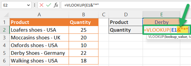
3. Enter an ampersand sign and an asterisk sign. Make sure to enter the asterisk sign within quotes. Otherwise, you will get an error.

The updated VLOOKUP function is;

=VLOOKUP(E1&”*”

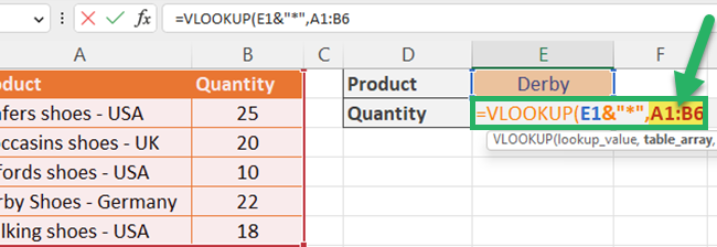
4. Select the lookup table. You can select a range or a named range.

In this example, you have to select the cell range A1:B6.

Then, your updated wildcard VLOOKUP function is;

=VLOOKUP(E1&”*”,A1:B6

5. Next, enter the column number from where you want to get the return value. In this case, you need to get the quantity and it is in the second column of the table.

Therefore, you have to enter 2 as the column index number.

=VLOOKUP(E1&”*”,A1:B6,2

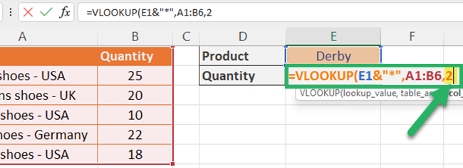
6. Select False as you want to do an exact match.

Now, your VLOOKUP wildcard function should be;

=VLOOKUP(E1&”*”,A1:B6,2,FALSE

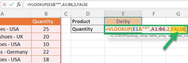
7. Finally, close the parentheses and press enter.

Your final VLOOKUP wildcard function should be;

=VLOOKUP(E1&”*”,A1:B6,2,FALSE)

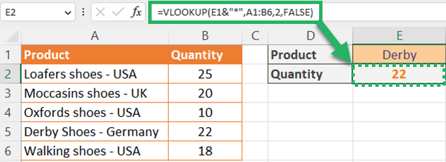
So, you will get the quantity for Derby shoes which is 22.

VLOOKUP wildcard formula example #2: Question marks as wildcards

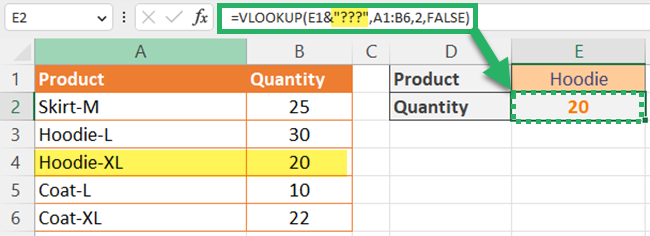
In the below data set, different products are given with the available quantity.

Assume that you want to find the quantity of any given product in Cell E1 with XL size.

If you use the asterisk sign as the wildcard character for the partial match in the above case, you will get the quantity for Hoodie-L.

The reason is that the asterisk sign represents zero or any number of characters. Hoodie-L is the first partial match for your VLOOKUP wildcards function.

So you have to do a partial match with a specific number of characters.

Then, you can use question mark wild character.

One question mark represents only one character. If you want to specify two characters, you have to use two question marks, and so on.

In the above example, there are three characters after the main product name including the hyphen sign.

Pro Tip:

If there are trailing spaces you have to remove those. Otherwise, the function will not work as expected.

Because spaces also count as characters.

Therefore, you have to enter three question marks as wildcards for the VLOOKUP function.

The VLOOKUP function is the same as the previous example, except for the lookup value.

So, your formula should be;

=VLOOKUP(E1&”???”,A1:B6,2,FALSE)

VLOOKUP wildcard formula example #3: Tildes as wildcards

The below data contains the full name of each employee and their contribution to the total sales amount.

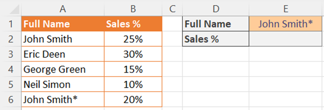
Two workers name “John Smith” work for the above company. To identify them, an asterisk is used for John Smith, who recently joined👬

You must now find the sales contribution from John Smith, who recently joined.

If you use a conventional VLOOKUP function in this example, you will get “John Smith’s” sales contribution.

The reason for this is that VLOOKUP treats the asterisk as a wildcard character.

The tilde can be used to cancel off the impact of the asterisk.

Then, your VLOOKUP should be;

=VLOOKUP(E1&”~*”,A1:B6,2,FALSE)

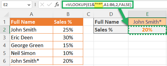
The tilde nullifies the effect of the asterisk sign.

Then, the VLOOKUP wildcard function returns 20% as John Smith*’s contribution to total sales.

That’s it – Now what?

Great work! 🎉 Now you know how to use wildcard VLOOKUP functions and make VLOOKUPs more powerful.

But VLOOKUP is just one of the commonly used Excel functions.

There are still more core Excel functions that can powerfully help you 💪

Are you curious about other functions that can powerfully help you just like the VLOOKUP?

Learn more about the VLOOKUP, together with the IF and SUMIF functions when you join my free 30-minute online course 🚀

Learn Excel the way you want–fast, easy, and FREE 😊

Other resources

You can read our articles about VLOOKUP, and VLOOKUP in Excel VBA to master this function.

If you are a Microsoft Excel 365 user, you can replace the VLOOKUP function with the XLOOKUP function 🤩

Don’t forget to read our article How to Use Wildcards in Excel, if you like to know how to apply wildcard characters for other Excel functions.