4 Quick Ways to Wrap Text in Excel
By default, a cell in Excel is 15 points tall and 8.43 points wide. The said size is perfect to fit in numbers.
However, you might find yourself in situations where you would want to fit text in a spreadsheet. Particularly, if those are long sentences, it might be difficult for you to neatly fit them into a cell. 🤫
That is where you need the Wrap Text feature of Excel. To learn all about it – continue reading the article it follows.
Download our free sample workbook here to tag along with the guide.
Table of Contents
What is the Wrap Text feature in Excel?
There are two ways how the data in a cell that’s large enough to fit in might appear in Microsoft Excel.
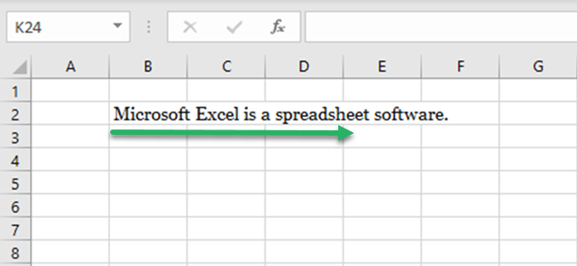
1. The text exceeds the boundaries of a cell, and the adjacent cell is empty. In such a case Excel lets the text string exceed the boundaries of the cell.
2. The text exceeds the boundaries of a cell, and the adjacent cell is not empty. In such a case Excel cuts off the text at the cell boundary.
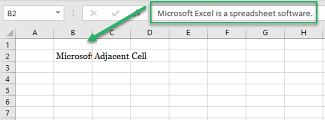
The Wrap Text feature of Excel is meant to save you from situations like these.
The sentence in the above image is too large to fit in a default-sized cell. To fit it in the cell, you may resort to dragging and dropping the column and the row.
But what if you have many such cells in Excel with texts of varying lengths?
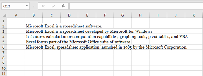
You don’t waste a whole evening resizing each column and row to perfectly fit the text in each. To do this in one go, Excel offers the Wrap Text feature.
Where hitting a single button would align it all for you!
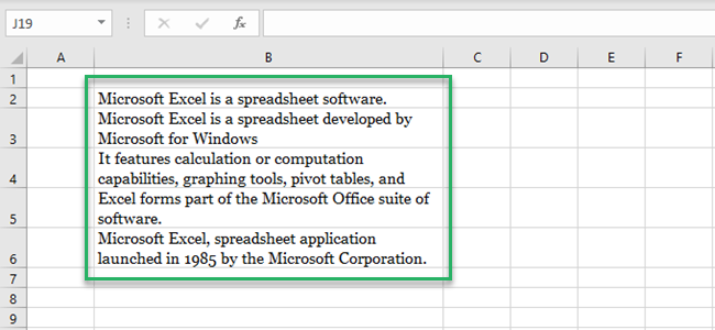
How to wrap text in Excel? There are four quick ways how you can wrap text automatically and manually in Microsoft Excel.
It’s time we see them one by one.
1) Wrap Text from the Ribbon
Excel Ribbon offers a ready button to wrap text in Excel.
Take the cells in the image below.

1. Select the cell/cells where you want the Wrap Text formatting applied.

This will be the cell that contains the text.
2. Go to Home Tab > Alignment Group > Click Wrap Text

3. And that’s it.
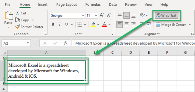
Wrapping text in Excel is a piece of cake!😀
2) Wrap Text using Hotkeys
Sometimes, you might be working in the ‘keyboard mode’ and simply don’t want to switch to a mouse or a joystick.
That’s alright. You can still wrap text automatically in Excel using hotkeys.
1. Select the cell/cells where you want the Wrap Text formatting applied.

Press Alt. This will activate the hotkey buttons on the Ribbon.
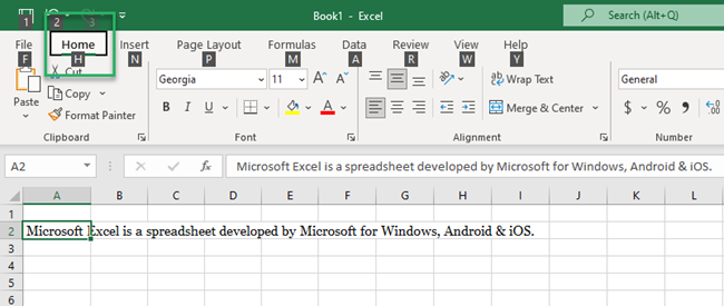
2. Next press ‘H’ to go to the Home Tab.
3. Press ‘W’ for Wrap Text.
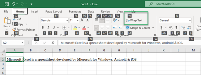
And there you go!

3) Wrap Text from the Format Cells Dialog Box
Another way to wrap text automatically in Excel is through the Format Cell Dialog box.
1. Select the cell/cells where you want the Wrap Text formatting applied.

2. Go to Home Tab > Alignment Group > Click the arrow button to the bottom right

Here’s a keyboard shortcut for you! Hit ‘Ctrl + 1’ to launch the ‘Format Cells’ dialogue box.
3. From the Format Cells popup menu:
Go to Alignment Tab > Text Control > Wrap Text
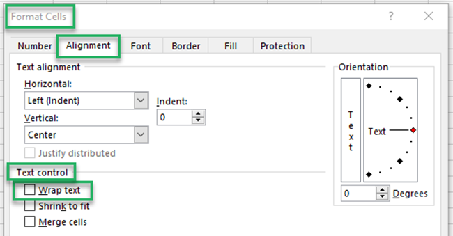
Here are the results!

All of the methods above automatically adjust the row height/column width to fit in the contents of a cell.
You might also choose to do this manually.
4) Wrap Text manually
There are two ways how you may manually fit the text into a single cell in Excel.
i. By adjusting the rows/columns
1. Select the column header where the text resides.
2. Hover your cursor over the boundary of the header to see a double-headed arrow.
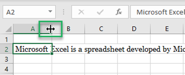
3. Hold it and drag it to change the cell size till you have reached the desired column width.

Or, if you do not want to resize the cell in terms of width but height, you may do the same for rows.
However, if you merely resize the row as above, it won’t work.

To fit the text in the cell, you not only need to resize the row but apply Wrap Text too.

ii. By adding line breaks
Line breaks in cells in Excel are just like ordinary line breaks that you’d add to any text of yours.
You can fit text in a cell in Excel by adding a manual line break.
1. To add a new line in a cell, double click the cell. This will activate the cell for writing to it.
Pro Tip!
Alternatively, you can use the keyboard shortcut of pressing F2 to activate a cell for editing. Or you can edit it from the formula bar. ✌️

2. Take the cursor to the position where the text exceeds the boundaries of the cell.
3. Press Alt + Enter to go to add a line break.

This breaks the line into two to help it fit in the cell.
This is not a very handy way to fit text in a cell in Excel because it leads to distortion every time a slight change is made.
iii. By applying AutoFit to Columns / Rows
Another way to fit text in a cell in Excel could be by applying the AutoFit settings to a cell.
1. Select the subject cell.
2. Go to Home Tab > Cells > Format > Auto Fit Row Height.

This is applicable if you want the height of the cell to be adjusted for fitting the contents.
3. Or Go to Home Tab > Cells > Format > Auto Fit Column Width.

This should help you if you want the width of the cell to be adjusted for fitting the cell contents and not the height.
How to remove Wrap text from Excel?
Unwrapping text in Excel is as easy as it is to wrap text in Excel.
Simply select the cells where you no longer want the wrap text feature applied.
1. Go to Home Tab > Alignment Tab > Click Wrap Text.
2. Or use the hotkeys by pressing Alt + H + W.
3. The Wrap text settings (if already applied) will be removed.
The same steps used to apply the wrap text can be reapplied to remove the wrap text formatting.
Bonus: How to wrap text in Excel Online
To wrap text in Excel Online, you can follow these steps:
- Open your Excel workbook in Excel Online.
- Select the cell(s) where you want to wrap text.
- Go to the “Home” tab on the ribbon.
- Look for the “Wrap Text” button in the “Alignment” group. It typically shows an icon representing lines of text with a wrap indicator.
- Click on the “Wrap Text” button. This will apply text wrapping to your selected cell(s), making all the content visible within the cell by increasing its height and wrapping the text across multiple lines within the same cell.
If you don’t see the “Wrap Text” button immediately, make sure you’re in the “Home” tab, as the Excel Online ribbon can be a bit different from the desktop version.
That’s it – Now what?
In the article above, we came across different methods on how to wrap text in Excel. Starting from the Wrap text button on Excel Ribbon, to hotkeys, to Format cells.
Not only these, but we also saw how you can manually adjust the size of a cell to fit its contents.
The Wrap text feature of Excel is going to save your spreadsheet from taking a terrible shape. However, Excel is not only about formatting but manipulating numbers.
The three most used functions of Excel include the VLOOKUP, SUMIF, and IF functions. Click here to sign up for my free 30-minute email course that is designed to teach you these functions (and more!).
Conclusion
Auto-fitting the height/width of cells in Excel is much more than what has just been explained above. Learn everything about auto-fitting the row height/column width of cells in Excel here.
Also, if this article interests you, we suggest you give a read to our other articles on using Format Painter in Excel, inserting a Digital Signature in Excel, and copying/pasting in Excel (formulas, values, and everything).
