How to Autofit in Excel – Step-by-Step Tutorial (2024)

By default, all the rows and columns in Excel take a uniform height and width.

However, Excel allows you to adjust the size of rows and columns to your choice.

And if you are short on time to manually adjust the size of each row and column – there’s an autofit feature to help you get through. 😀

The autofit feature of Excel automatically adjusts the size of rows and columns to fit the contents inside.

To learn how to use the autofit feature in Excel, let’s dive straight into the article below.

Download our free sample workbook here to follow the examples in the guide below.

How to autofit columns in Excel

Microsoft Excel offers two ways to autofit columns in Excel.

Autofit using the mouse:

To autofit column width in Excel using the mouse:

1. Click on the targeted column header.

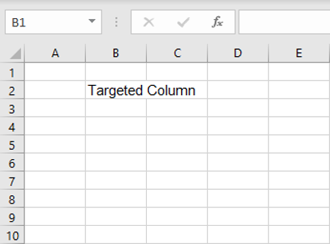
Doing so will select the entire column.

2. Hover your cursor over the right boundary to this column until a double-headed arrow appears.

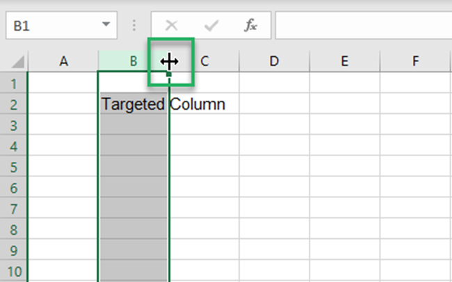
3. Once you have the double-headed arrow appearing, double-click to autofit the column width.

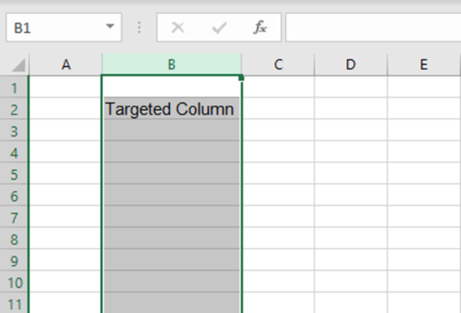
And there! Excel resized the width of the target column to match the size of the contents inside the column.

To apply the same to multiple columns:

1. Select multiple columns.

2. Hover your cursor over the boundary of any column within the selected range until a double-headed arrow appears.

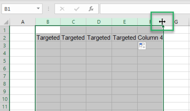
3. Once you have it, double-click to auto-fit the width of all the selected columns.

Excel will fix column width for all the selected column widths.

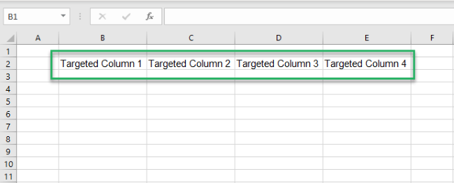
Autofit using the ribbon:

To autofit the column width in Excel using the ribbon:

1. Click on the targeted column headers to select the columns.

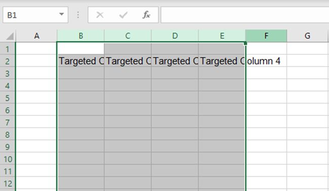
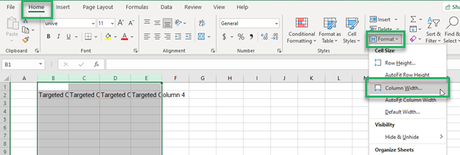
2. Go to Home > Cells > Format > AutoFit Column Width.

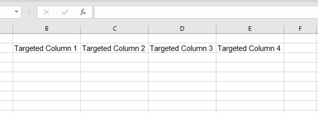
Excel autofits the width of the subject columns. 🙂

How to autofit Excel rows

Just like the autofit feature for columns, Excel offers two ways to autofit rows too.

Autofit using the mouse:

To autofit the height of an Excel row using the mouse:

1. Click on the targeted row header.

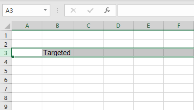
Doing so will select the entire row.

2. Hover your cursor over the lower boundary to this row until a double-headed arrow appears.

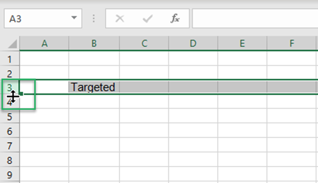
3. Once you have the double-headed arrow appearing, double-click to autofit the row.

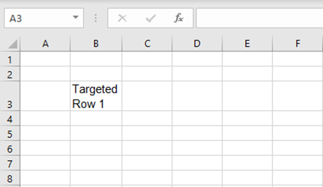
And there! The Row resizes to match the size of the contents inside the row.

To apply the same to multiple Excel rows:

4. Select multiple targeted rows.

5. Hover your cursor over the boundary of any row within the selected range until a double-headed arrow appears.

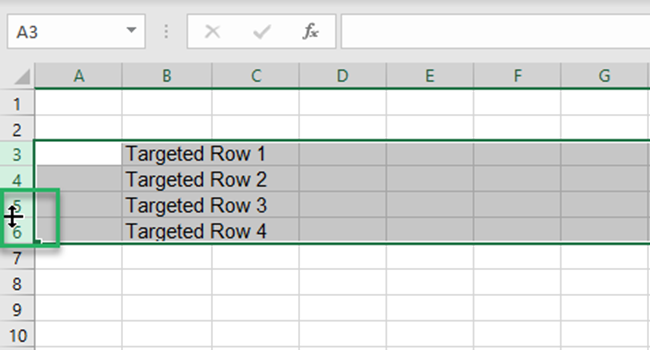
6. Once you have it, double-click to auto-fit the width of all the selected rows.

Autofit using the ribbon:

To autofit an Excel row using the ribbon:

1. Click on the targeted row header to select the entire row.

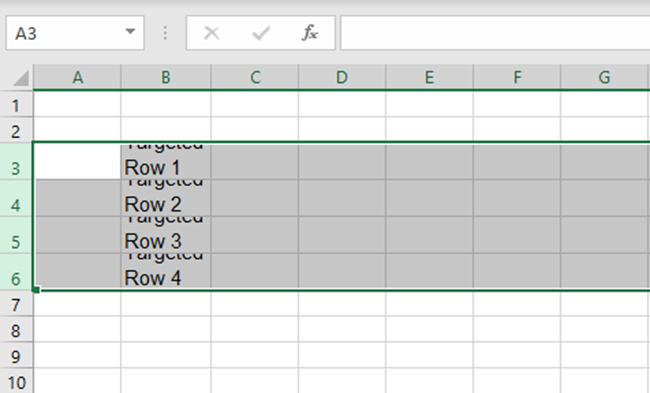
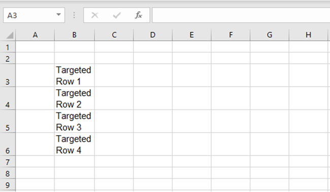
2. Go to Home > Cells > Format > AutoFit Row Height.

Excel autofits the height of the subject rows.

How to change cell size

A cell is formed at the intersection of a row and column.

So, to change the size of a cell, you need to change both the size of the row and the column.

For example, let’s take the example below.

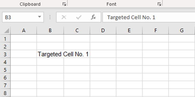
The cell in the image above has text that doesn’t fit into the cell.

1. Select the cell.

2. Go to Home > Cells > Format > Cell Size > Row Height.

This opens the dialogue box as shown below.

3. In this box, punch in the required row height.

We are setting the height to 30.

This adjusts the height of the cell as follows.

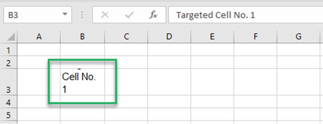
4. Next, let’s adjust the width of the column.

5. Go to Home > Cells > Format > Cell Size > Column Width

This opens the dialogue box as shown below. To change the column width, punch it in.

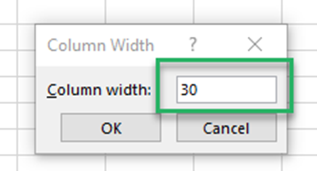
6. In this box, punch in the desired column width.

We are setting the width to 30.

This changes the width of the cell as follows.

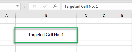
That is how you can fix the size of any cell as required. ✌️

Another easy way to do this can be doing it by adjusting the boundary using the mouse.

1. Select the row header (where the cell is situated).

2. And hover the cursor around the boundary until the double-headed arrow appears.

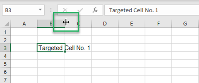
3. Drag it till the height of the row is adjusted as required.

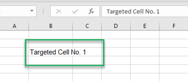
4. Next, select the column header (where the cell is situated).

5. And hover the cursor around the boundary until the double-headed arrow appears.

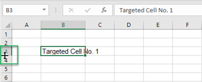
6. Drag it till the width of the column is adjusted as required.

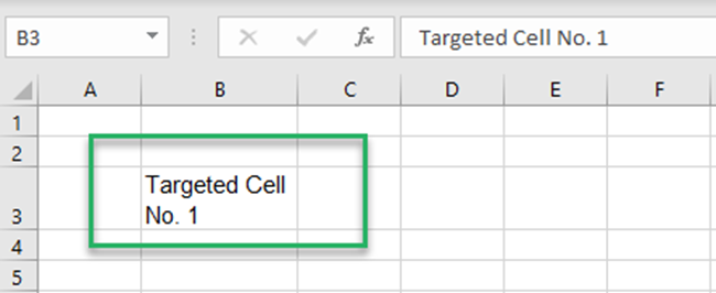
And there you go!

How to make all cells the same size

To make all cells the same size in Excel, follow the steps below.

1. Press Ctrl + A to select the entire sheet (or multiple cells, if needed).

2. Alternatively, press the ‘All cells’ button to the top left of the worksheet.

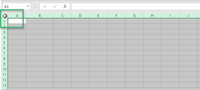
3. Go to Home > Cells > Format > Cell Size > Row Height.

In the row height dialogue box, punch in the desired number, say 30.

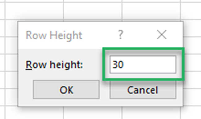
4. Next, Go to Home > Cells > Format > Cell Size > Column Width.

In the column width box, punch in the desired number, say 30.

Excel adjusts all cells’ height and width to one size (the specified size).

That’s it – Now what?

If you have come this far, you already know how to autofit rows and columns in Excel. In the above article, we also learned to change the cell sizes and to make all cells of the same size.

While these things will be of great help to you in shaping your Excel spreadsheet – this is only about formatting in Excel.  To make the best use of Excel, you must have a good grip on the core functions of Excel.

Like the three fundamental functions of Excel including VLOOKUP, IF, and SUMIF functions.

Click here to sign up for my free 30-minute email course that will take you through these functions (and more!).

Other resources

Knowing formatting shortcuts in Excel will expedite your work in Excel.

If you find the above article interesting,  you’d also love other similar articles. Check out our blog on wrapping text in Excel and hiding / unhiding rows and rows in Excel.