How to Get Absolute Value in Excel With the ABS Function
We live in a world of numbers. 🤔
A number can take two types – it can be positive or negative. The sign to a number can make a great impact on your calculations.
And what if you only need positive numbers? The ABS function of Excel saves the hassle of redoing the negative values to positive ones.
That’s what we call finding absolute value in Excel. Learn all about it in the article that follows.
And do not forget to download our free sample workbook here to practice the examples below.
Table of Contents
How to get absolute value with the ABS function
In the simplest of words, an absolute value is the positive value of a number.
A number may be positive (like 5) or negative (like -5). The absolute value for both numbers is a positive 5.
The image below has a list of numbers.
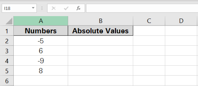
We can see the list has positive and negative values.
Positive values bear no sign. Whereas negative values may be prefixed by a minus sign. Or, under different number formatting in Excel, they might be enclosed in parenthesis.
Can we have them all turned into absolute (positive) values? Here are a few examples: 😯
1. Write the ABS function as follows.
= ABS (A2)
The referenced cell (A2) contains the value that we want to be converted into an absolute value.Steve Jones”. That means the lookup value has 2 matches in the lookup column.
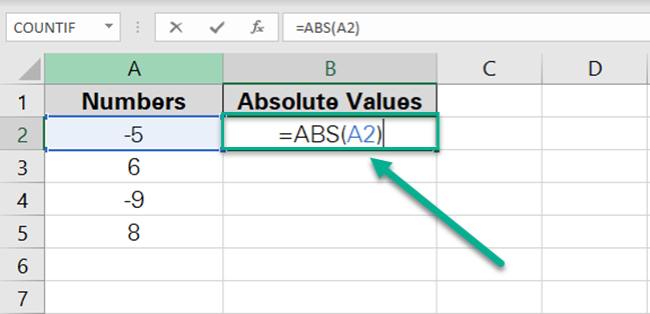
2. Excel turns the value of cell A1 into an absolute value. A positive 5.
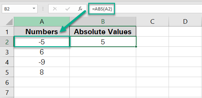
To find absolute values for all the other numbers too, drag and drop cell B2.
And here come the absolute values.
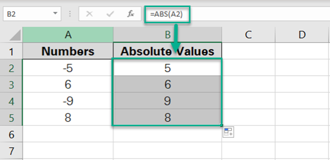
Must note the absolute value of a positive value is still positive. The absolute value for positive 6 in Cell A5 is still positive 6.
Formula example: ABS and SUM
The ABS function becomes the most useful when used in pair with another function. Like the SUM function.
Let’s continue with the same table as above

We want to find the sum of these values. But only by taking them all as positive values.
1. Write the ABS function as follows.
= ABS (A2:A6)
This function tells Excel to convert the values of Cell A2:A6 into absolute values.
Pro Tip!
If you run the ABS function with a range of cells specified like A2:A6, it will become an array formula. And the result would be an array of values.👍
2. Nest the above function in the SUM function as follows.
= SUM (ABS (A2:A6))
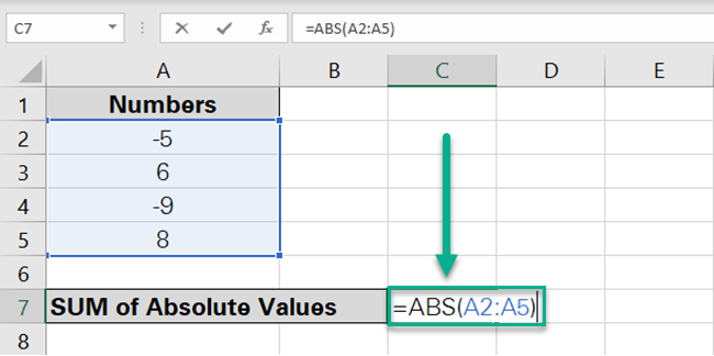
The formula says, ‘Turn the values of Cells A2 to A6 into absolute values and then sum them up.’
3. So here come the results.
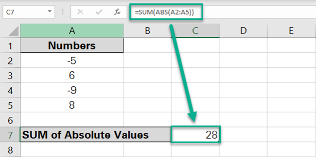
That is only one combination. You may use the ABS function for multiple calculations of the like nature.
Like the Product, Exponent, Division, SUMPRODUCT function, and whatnot.
Use-case example: Sort values by absolute values
If you’ve read this article until here, you’d now know how to use the ABS function.
However, are you still wondering why you may even need the ABS function? That’s a common thought, and that’s alright.
The data below shows some transactions made from a bank account.
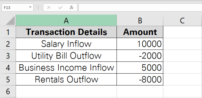
Some of them are positive (that shows cash inflow), and others are negative (cash outflows).
You quickly want to sort all these positive and negative numbers in descending order to find out the most significant transactions.
1. If you apply the simple SORT function:
=SORT (A2:A6, , -1)
The first argument tells the range to be sorted. The second argument is omitted. And the third argument is set to -1 (to denote descending order).
2. The results would be as follows.
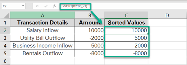
Excel sorts the data from the biggest positive number to the biggest negative number. Like we see numbers on a number line.
This takes a bigger transaction amounting to $8000 to a lower position. And ranks a smaller transaction of $2000 transaction above.
That was not what we wanted.
3. To have the transactions rightly sorted, nest the ABS function in the above formula.
=SORT (ABS(A2:A6), , -1)
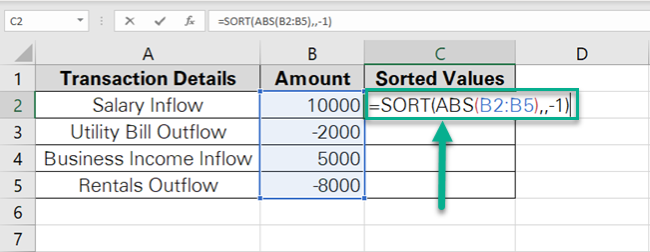
The listing now changes.
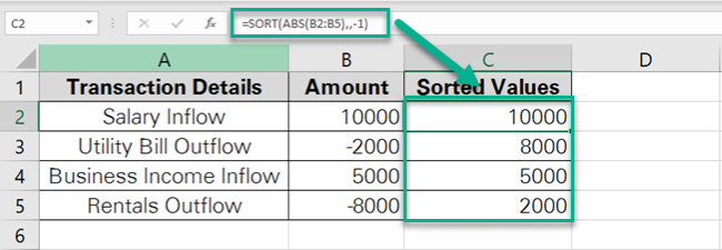
This time all the transactions are sorted rightly (in terms of the monetary amount). Signs of the amounts are ignored.
That’s it – What’s next?
That’s all about the ABS function of Excel. Easy, isn’t it?
If you didn’t know about the ABS function already, the above article must have helped you master it.
The ABS function of Microsoft Excel might not be much useful in itself. But, when combined with other functions of Excel like the VLOOKUP, SUMIF, and IF functions, it can ease your work to a great extent.
Want to learn how to use these functions?
Click here to enroll for my 30-minute free email course and learn them (+ pivot tables) in no time.
Other resources
The ABS function can come to your rescue in many situations.
Some of the times, you are not really looking out for absolute values but a different visual representation of the same value.
If that’s the case, check out how to format numbers in Excel.
