Excel SORT Function: Sort Excel Data Using a Formula (2024)

When we are working in Excel, sometimes we need to sort data. It helps us organize and analyze data, find patterns, or highlight important information 💡

You can use Excel’s SORT function to sort your data in ascending or descending order.

It is one of the dynamic array functions in Excel but there’s a lot more that it can do 😀

In this article, you will learn how to use the SORT function to sort data in one or more columns in Excel.

You can download the attached Excel workbook to practice this function.

How to use the SORT function

Excel SORT function sorts data of range or array in desired sort direction.

The below table shows the sales details of each employee with their region 💰

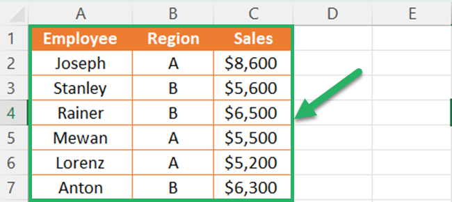
Assume that you want to extract employee names in the above table to a new column and sort them in ascending order.

You can sort a range using the below steps.

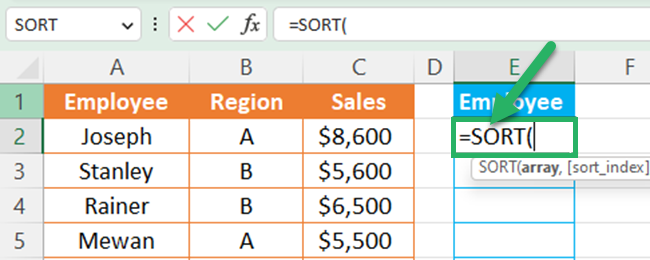
1. Enter an equal sign and select the SORT function.

So, your formula bar should show;

=SORT(

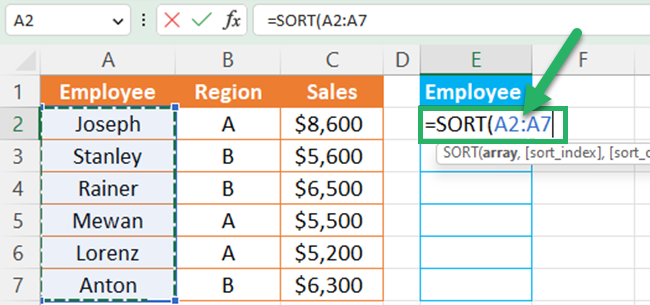
2. Select the cell range to sort. In this case, you have to select the employee name range.

Now, your formula should be;

=SORT(A2:A7

3. Close the parentheses and press the Enter key.

All sorted names will be shown in the new column.

Your final formula is given below.

=SORT(A2:A7)

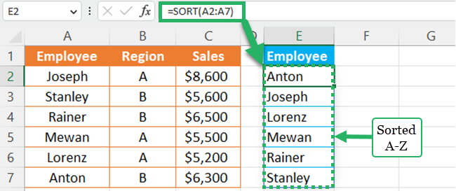
Excel sorts text values in alphabetical order by default. Therefore, in the above example, employee names (one column) are extracted to a new column in ascending order.

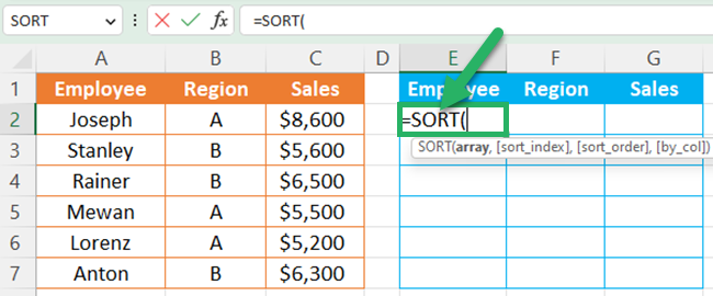
If you want to get all columns of a table to a new cell range by sorting in ascending order based on the first column, you can apply the below steps.

1. Enter an equal sign and select the SORT function.

So, your formula bar should show;

=SORT(

2. Select the cell array to sort. In this case, you have to select the cell array of the table.

Now, your formula should be;

=SORT(A2:C7

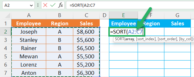
3. Close the parentheses and press the Enter key.

The entire data table will be sorted in ascending order based on the first column.

Your final formula is given below.

=SORT(A2:C7)

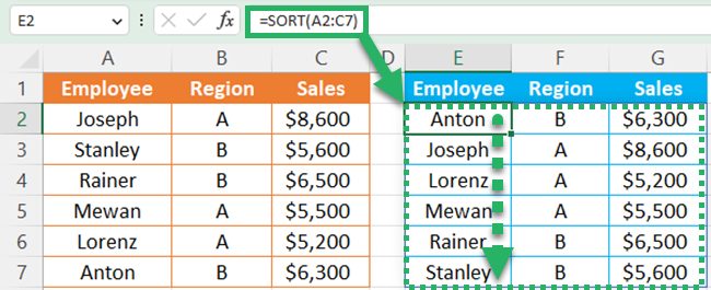
Now, there is a separate table with sorted data based on the first column.

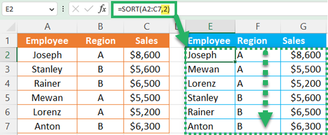
Assume that you want to sort the entire table based on the Region. Then, you have to specify that you must specify the second column in the second argument.

So, your column index should be 2.

The updated formula should be;

=SORT(A2:C7,2)

Pro Tip:

You can keep the SORT function’s first argument as a dynamic array if you keep the source data as an Excel Table.

Then, even when you add a new column or new row it will automatically update the SORT function 🥳

Otherwise, you have to manually adjust the array argument in the SORT formula.

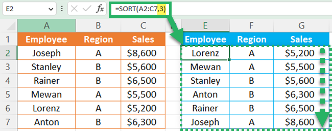
Similarly, if you want to sort the entire table based on the sales column (third column), you have to enter 3 as the column index.

So, your formula will be;

=SORT(A2:C7,3)

Pro Tip:

Do you want to sort by multiple columns at once with the SORT function?

You can do that as well 🤔

For that, you have to use an array constant for the column index.

If you want to sort the above data first by Region and then by Employee name you can enter the below formula.

=SORT(A2:C7,{2,1},1)

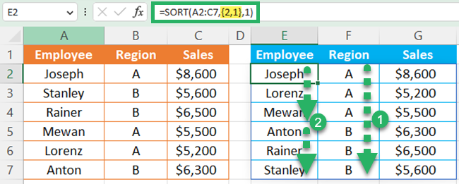
Using the above formula, first, the region column is sorted alphabetically. Then, the employee column is sorted alphabetically 😍

In all the above cases, you got a sorted list of source data in ascending order.

You can use the SORT function to sort data in descending order as well 🤠

For that, you have to use the third argument of the SORT function.

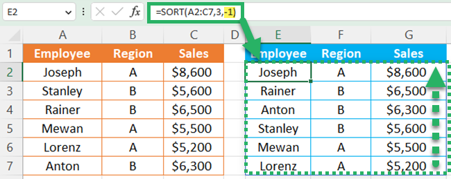
Say that you want to sort data based on the sales values and you want to get the highest sales values to the top of the list.

Then, you have to sort columns in descending order.

You can add -1 as the third argument to sort data in descending order.

So, your sort formula is;

=SORT(A2:C7,3,-1)

Pro Tip:

The Excel SORT function is a dynamic array function. However, the SORT function references a column index number. If you add or delete columns, your sorted data will be distorted.

For Example, if you add a new column to the source array of the above example, your output will be changed like below.

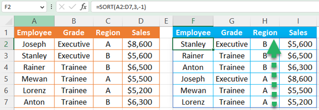
Now, column index 3 is “Region” in the source data. Therefore, the array will be sorted based on the “Region” instead of “Sales” values.

If you need to sort data in a grid, it is better to use the SORTBY function because it references a range to sort. You have to select the column you want to sort. Then, your sorted data will not be affected due addition or deletion of columns in the source data.

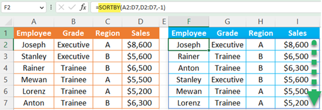
The SORTBY function helps to sort by more than one column as well.

By default, the SORT function sorts data by rows.

If your data table is arranged horizontally, then you cannot sort data by rows.

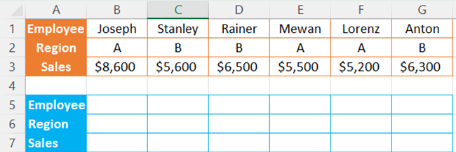
In such cases, you have to sort by columns.

You can use the last argument -“By_col” to sort your data by columns.

If you want to sort the above data in descending order by sales values, follow the below steps.

1. Enter an equal sign and select the SORT function.

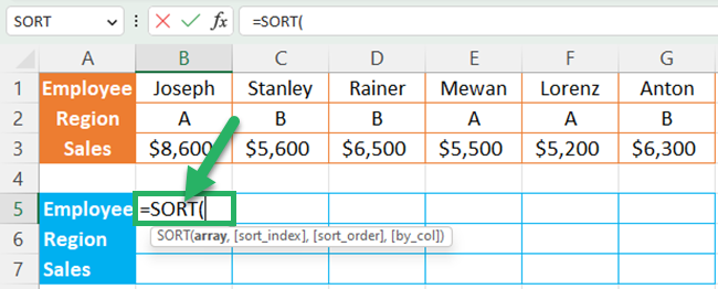
2. Select the data array.

Now, the formula is;

=SORT(B1:G3

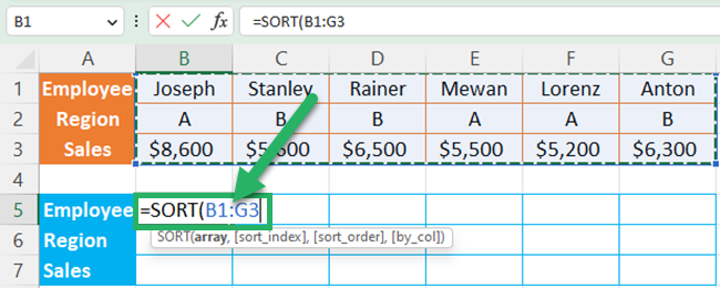
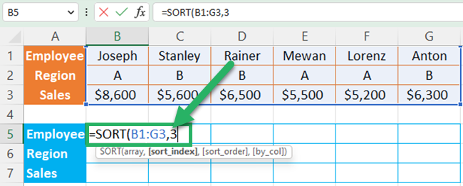
3. Enter the sort index. The first Row – “Employee” is 1, the second row – “Region” is 2, and the third row – “Sales” is 3. So, you have to enter 3 as the sort index.

Then, your sort formula should be;

=SORT(B1:G3,3

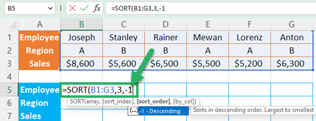
4. Enter -1 to the third argument of the SORT function to sort in descending order.

You can see the below formula in the formula bar.

=SORT(B1:G3,3,-1

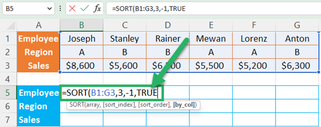
5. Select TRUE for the last argument of the SORT function to sort by row.

The updated SORT formula is;

=SORT(B1:G3,3,-1,TRUE

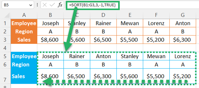
6. Finally, close the parentheses and press “Enter”.

The formula for the final result is;

=SORT(B1:G3,3,-1,TRUE)

The SORT function can be combined with other functions as well.

SORT + UNIQUE and SORT + FILTER are common examples.

SORT + UNIQUE formula example

When you apply the UNIQUE function to get unique values, you can do sorting data using the SORT function.

You are given the below sales table.

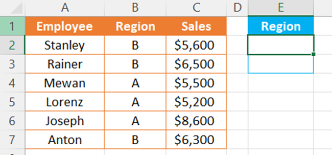
Now, you need to find the what are the regions in the above sales table.

If you directly apply the below UNIQUE function, return values that are unique for the region column. But, it will not be sorted 😢

=UNIQUE(B2:B7)

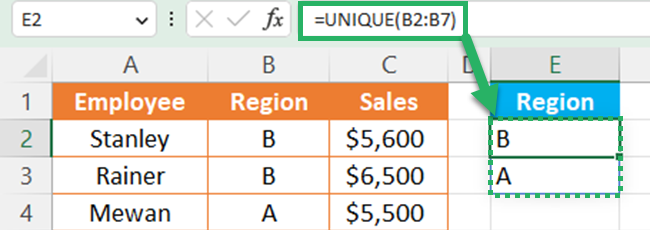
To sort alphabetically your unique list, you can combine the UNIQUE function with the SORT function 😊

=SORT(UNIQUE(B2:B7))

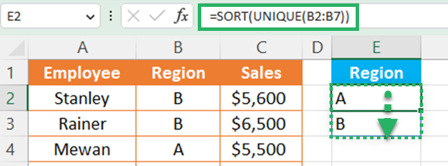
Now, the Excel SORT function sort values of the UNIQUE function results.

That’s it – Now what?

Well done! 👏 Now that you know how to use the SORT function in Excel, you can easily organize and analyze the data in your spreadsheets.

But that’s only the basic things Excel can do. You can unlock the full potential of Excel by learning Excel VBA.

With VBA, you can just double-click on the headers and sort your data in Excel. 🤯

Learn how to record and edit macros easily and for free when you enroll in my 30-minute online course. I promise you, it’s not as hard as you think.

Other resources

If you want to refresh your knowledge about sorting data in Excel, read our article about how to sort in Excel.

When you are working with Excel functions, it is common to sometimes get Excel errors.

You can read our Excel errors article to learn how to fix those 😊

Frequently asked questions