SUMPRODUCT in Excel: How to Use It with Easy Examples
The SUMPRODUCT function is one of Excel’s math and trigonometry functions.
The SUMPRODUCT function multiplies the corresponding values of two or more ranges and gets the total of that.
Most Excel users know only this basic use of the SUMPRODUCT function 😟
But the SUMPRODUCT function is a far more handy function than you think 🤔
You can replace many Excel functions directly with SUMPRODUCT.
In this tutorial, we are going to explore the Excel SUMPRODUCT function.
You can download the attached Excel workbook to practice.
Table of Contents
How to use SUMPRODUCT
First, we will learn how to use the SUMPRODUCT function in a basic way 🙂
I have a data set in which we want to calculate total sales.
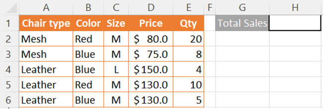
In this case, we want to calculate total sales without a sales column.
You don’t need to multiply each product’s price and quantity and then add all the sales together.
The SUMPRODUCT function in Excel calculates all these for you.
You can follow the below steps to apply the SUMPRODUCT function.
- Enter an equal sign and select the SUMPRODUCT function.

- Select the first array. To get total sales, you have to multiply the corresponding values in the price and quantity columns.
So, you can select column D as the first array.
Now, the following formula can be seen in the formula cell.
=SUMPRODUCT(D2:D6

Excel SUMPRODUCT function treats non-numeric values in the given array as zeros.
- Select the quantity values as the second array of SUMPRODUCT.
So, in this case, it’s the values in column E.
All arrays must have the same dimensions.
If not, the SUMPRODUCT function returns #VALUE! error value.
Now, the updated SUMPRODUCT formula with two arrays is;
=SUMPRODUCT(D2:D6,E2:E6

You can select one or more ranges to SUMPRODUCT function, but up to 255 arrays.
If you have selected only one array for the SUMPRODUCT function in Excel, you will get simply the SUM of that array.
You have to select only column E values to get the total of the quantity column.
Then, your SUMPRODUCT formula is;
=SUMPRODUCT(E2:E6)

- Close the parentheses and press “Enter”.
The final SUMPRODUCT function is;
=SUMPRODUCT(D2:D6,E2:E6)

Wow! The total sales value is ready! 🥳
Pro Tip:
You can replace the commas that separate array arguments with arithmetic operations.
You have to just enter each argument in parentheses and use the arithmetic operators in the actual formula.
In this case, sales equal the price multiplied by the quantity.
So, your SUMPRODUCT formula is;
SUMPRODUCT((D2:D6)*(E2:E6))
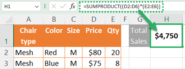
You can use this method to get the conditional sums in the next section.
SUMPRODUCT and IF: Sum with condition
Excel 2003 and older versions don’t have SUMIFS, COUNTIF, or AVERAGEIF functions.
Those times the SUMPRODUCT function handles all of those functions.
Even today, you can use the SUMPRODUCT function to calculate data with conditions 🎉
The SUMPRODUCT function can handle logical tests inside arrays.
With logical tests, the SUMPRODUCT function will get true and false values.
You can learn this using the below example.
Assume that you need to get the total sold quantity of Size “M”.
- Enter an equal sign and select the SUMPRODUCT function.
Now you can see,
=SUMPRODUCT(

- Open a parenthesis and select the cell range in the size column.
In this case, it’s the values in column C.
Now, the SUMPRODUCT formula is;
=SUMPRODUCT((C2:C6

- Enter the array parameters and close the parenthesis.
You need to get the quantity if the size is equal to M and it is given in cell H3.
so, you have to type the condition as =H3.
Now the updated SUMPRODUCT formula is;
=SUMPRODUCT((C2:C6=H3)

As this is a logical test, the result of the defined range will be converted to true and false values.
- Enter an asterisk * (multiplication operation in Excel) and select the numerical values in the quantity column.
Use parentheses for the cell range of quantity data.
Your formula bar will show;
=SUMPRODUCT((C2:C6=H3)*(E2:E6)

- Close the parentheses and press “Enter”.
=SUMPRODUCT((C2:C6=H3)*(E2:E6))
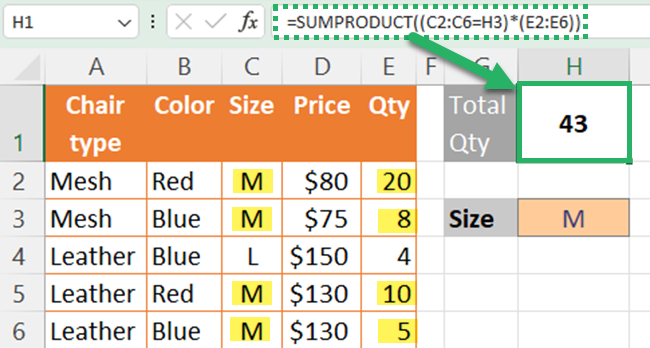
After you use the math operator (asterisk), Excel will automatically convert the true and false values to 1s and 0s. Excel will assign 1 if the value is true and false values will show as zeros.
In this example, the SUMPRODUCT function works like this.
=SUMPRODUCT((C2:C6=H3)*(E2:E6))
=SUMPRODUCT((="M")*(E2:E6))
=SUMPRODUCT(*(E2:E6))
=SUMPRODUCT(*)
=SUMPRODUCT()
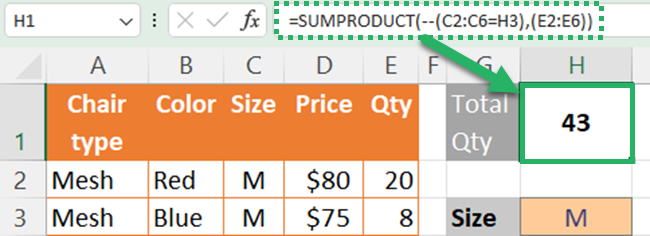
Do you want to select each array after a comma? ⚡
Then, each logical test inside arrays must start with a double negative sign ➖➖
So, in this case, the SUMPRODUCT formula is;
=SUMPRODUCT(–(C2:C6=H3),(E2:E6))
In the above example, you have used only one criterion.
You can use the SUMPRODUCT function for calculating data with multiple criteria also.
Say that you need to get the total sold quantity of chairs which are size “M” and color “Red”.
- Enter the same SUMPRODCT function which you have used for conditional sums with one criterion.

- Use an asterisk * (multiplication operation in Excel) and enter the second condition.
The color criterion is given in cell H4.
So, your updated formula should be;
=SUMPRODUCT((C2:C6=H3)*(E2:E6)*(B2:B6=H4)

- Close the parentheses and press “Enter”.
=SUMPRODUCT((C2:C6=H3)*(E2:E6)*(B2:B6=H4))
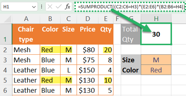
Now, you know how to get the sum with the condition using the SUMPRODUCT function in Excel.
You can use the SUMPRODUCT function for comparing data as well 😍
Then, you can replace it with the COUNTIF function.
In the below example, you have the product-wise budgeted and actual quantities.
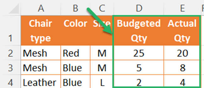
Now you need to find how many chair types have an actual quantity more than their budgeted quantity.
You can simply use the below SUMPRODUCT formula for comparing data.
=SUMPRODUCT((D2:D6<E2:E6)*1)
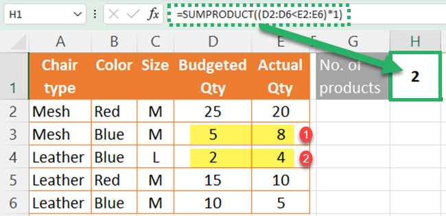
The SUMPRODUCT function compares corresponding values in the same row and returns true or false values.
When you multiply it by 1, true and false values will be converted to numeric values and you get the total of that as your count.
The SUMPRODUCT function in Excel can be used with other functions to get array formulas.
For example, LEN, ISBLANK, and ISTEXT functions are not array functions.
If you want to use the above functions for an array, simply combine those functions with SUMPRODUCT 🤩
You can practice the below example to learn that.
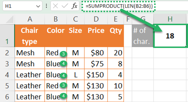
Assume that you want to know how many characters are in column B, color data.
You can enter the below formula for that.
=SUMPRODUCT(LEN(B2:B6))
That’s it – Now what?
Congratulations! Now you are an expert in one of the super Excel functions – SUMPRODUCT 🎇
However, SUMPRODUCT is not the only important function in Excel.
You must learn other functions like IF, and VLOOKUP functions to add more value to your Excel models.
You can enroll in my free 30-minute online course and learn them easily.
Other resources
If you want a Swiss army knife kind of function, you can replace SUMIF, COUNTIF, AVERAGEIF (and more!) with SUMPRODUCT.
Because SUMPRODUCT supports array operations directly for many Excel functions 🤗
It helps to keep your formulas compact too!
The XLOOKUP function in Excel is another powerful function in Excel 💪🏻
Read and learn how to replace VLOOKUP, HLOOKUP, INDEX MATCH, and many other Excel lookup functions.
