How to Alphabetize in Excel: Step-by-Step Guide (2024)

In a world where data is king, Excel remains the undisputed champion of organizing it.

And when it comes to sorting in Excel, there’s no better tool than the alphabetization feature.

So, whether you’re an Excel pro or just starting out, mastering the art of alphabetization in Excel is a must-have skill 😀

In this step-by-step guide, we’ll show you just how easy it is to sort your data alphabetically. You will be organizing your information like a pro in no time!

If you want to practice alphabetizing in real-time, download our sample workbook here.

Alphabetize A-Z or Z-A with the ‘sort’ feature

The quickest method to alphabetize your data is using the Excel Sort feature. It’s easy to use and only takes a couple of seconds. Let’s see how to use it below ⬇

Say, we have the following sample data.

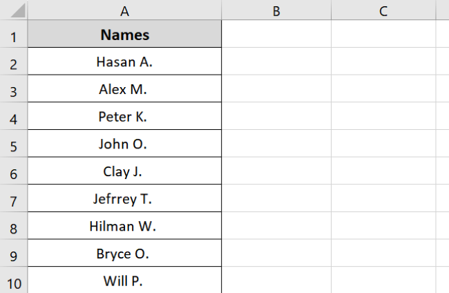
It contains the names of students of a class. We want to sort the names from A to Z to organize them.

To do that,

1. Select cell A1.

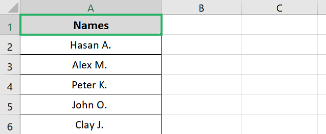
2. Go to the Data Tab and select the Sort option from the Sort & Filter group.

3. You can do the same from the Sort & Filter option under the Editing group.

4. Excel will alphabetize your list as follows:

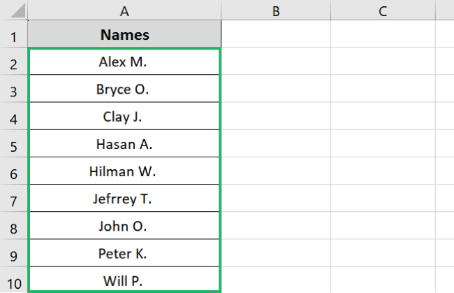
Pretty easy, no? 😉

Now, what would happen if we had multiple columns and had to sort them in alphabetical order?

It’s easy; we will only sort one column. The remaining columns will be sorted accordingly.

Want to see how? Read on.

Say, we have a sample data set.

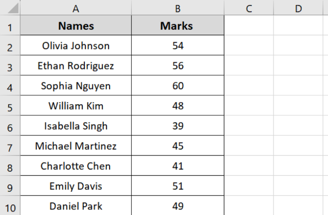
It contains information about the marks of students in a class in Mathematics. We want to sort both columns, but we will only sort column A.

Let’s see it in detail below.

1. Select cell A2.

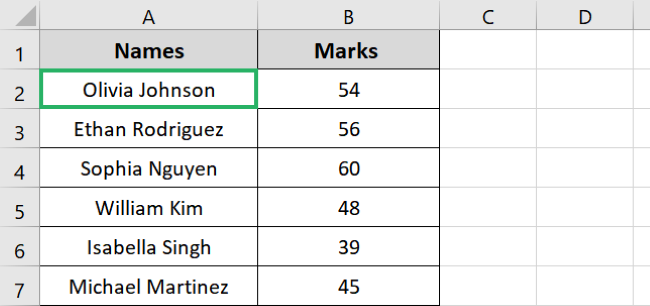
2. Go to the Data tab and select Sort.

3. Excel will automatically sort both columns.

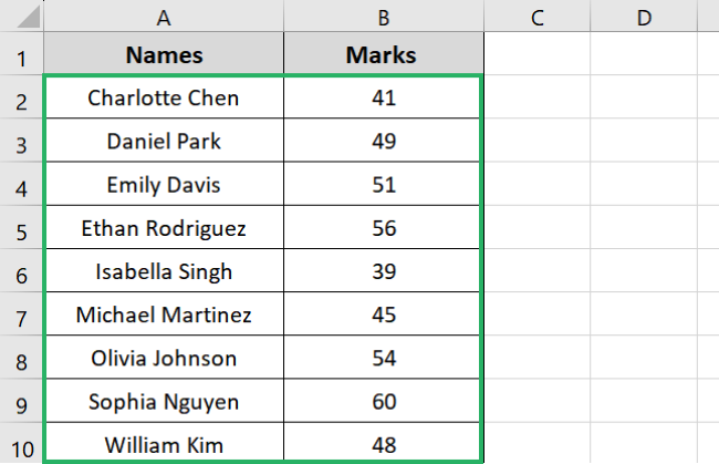
And it’s done. How cool was that! 🎯

Alphabetize with the filter button

Another method to alphabetize in Excel is by using the Filter button. This is more convenient to use as it combines all options and they are only a click away.

Adding a filter creates a dropdown for the selected column in the Excel spreadsheet. You can select different options from the dropdown menu easily 😃

Let’s see how to add a filter below.

Say, we have the following set of data.

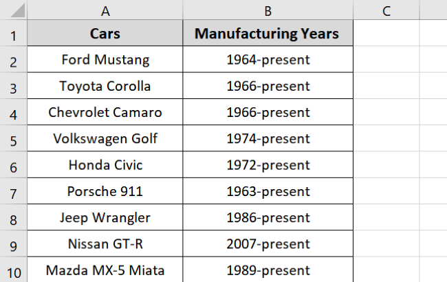
It contains information about some cars and their manufacturing years. We want to sort both columns in descending order 🔽

To do that,

1. Select both the column headers.

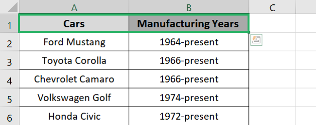
2. Go to Data Tab and Click Filter under the Filter group.

3. A small drop-down arrow will appear at the top of each column header.

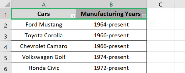
4. Click the arrows, and a drop-down menu will appear.
5. You can now select whichever order you want to alphabetize columns – we will select A to Z.

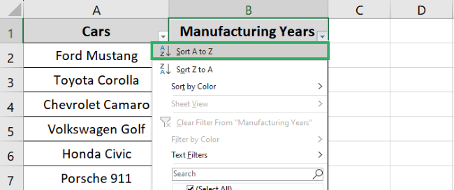
Excel sorts both the columns as:

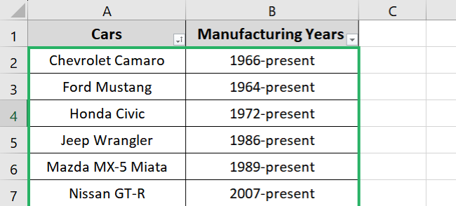
How quick was that? Try it yourself using the sample workbook provided 💪

Alphabetize with the SORT function

You can also alphabetize data in Excel using the SORT function. It works the same as other methods but is slightly more fun to use.

Before we use the SORT function, let’s have a look at its syntax.

=SORT(array, [sort_index1], [sort_order1], [sort_index2], [sort_order2], …)

The syntax might seem daunting 💀

But once you get a hold of it, it will be the most interesting method to use. Let’s understand the terms used below.

• array refers to the range you want to sort.
• sort_index1 is the row or column you want to sort. 1 refers to the first column, 2 to the second and so on.
• sort_order1 refers to the order you want to sort in, i.e., ascending or descending. Use 1 and -1 for ascending and descending, respectively.
• sort_index2 is the column you want to sort – by adding more levels.
• sort_order2 refers to the sorting order for the second level.

Let’s now use the SORT function to sort our data.

We have the following sample data.

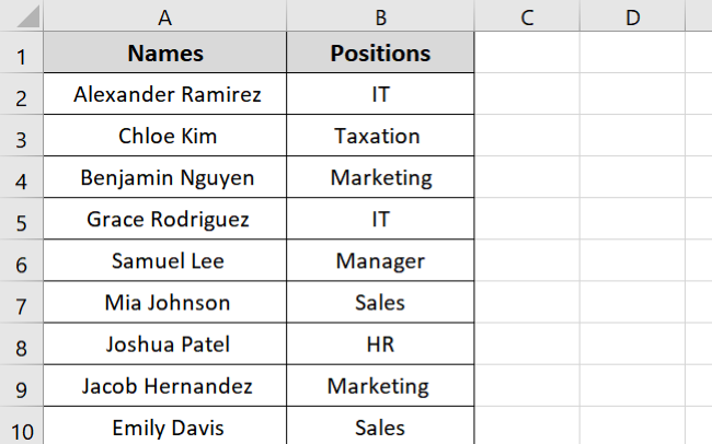
It contains information about the employees of a company and their positions. We will add a filter button to both columns and then sort alphabetically.

To do that,

1. Select cell C2.

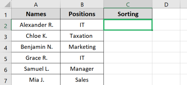
2. Enter the SORT function as:

=SORT(

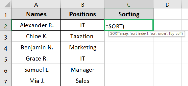
3. Enter the range to sort.

=SORT(A2:B10,

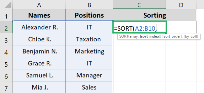
4. Enter the sort index – 1.

=SORT(A2:B10, 1,

5. Enter the sort order- in our case, -1.

=SORT(A2:B10, 1, -1)

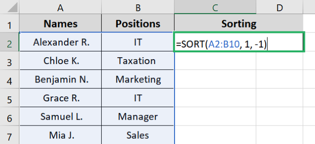
6. Press Enter.

And it’s done! 🥇

Column A has been sorted in descending order as:

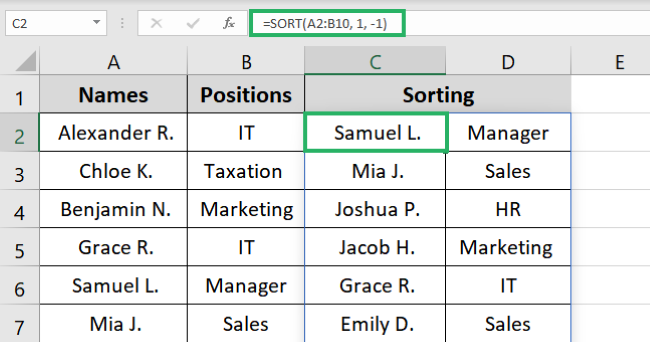
Pretty cool, no? 🤩

That’s it – Now what?

In this article, we saw how to alphabetize data in Excel. We saw how to perform the task using three different methods – the easiest of all is the sort feature.

Alphabetizing in Excel can be very helpful, especially when you have tons of data to organize. You can use any of the above-stated methods to sort your data.

Luckily, similar to alphabetizing data, Excel has a variety of other interesting features. The best of which are Excel functions 💻

Our favorite Excel functions include IF, SUMIF and VLOOKUP. You can learn them for free in my 30-minute free email course that teaches just this and more. So sign up now!

Other resources

Did you learn something new from this article? If yes, then you’d love to know more.

Try similar topics: Sort Data in Excel, Sort Function, Filter in Excel and more.

Frequently asked questions