How to Sort Columns in Excel
(Without Mixing Data)

When I say Excel is the most powerful spreadsheet software – that’s not an exaggeration.

Excel lets you do even the toughest of tasks with immense ease of use, let alone the simple ones. And what’s simpler than sorting data? Excel offers a plethora of options you can use for sorting data.

Whether you want to sort cells using their numeric values or background colors, with Excel, you can do it all 😉

This guide entails everything you need to know about sorting data in Excel. So without further ado, let’s get right into it.

You can only learn so much by reading stuff online. Practice sorting data in real time by downloading our sample workbook here.

Sort data based on one column

Sorting data in Excel is pretty simple – especially when working with a single column.

Say we have the following set of data.

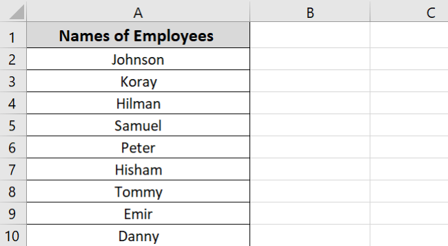
And we want to sort the name of employees in alphabetical order from A to Z.

All you need to do is:

2. Select the first column.
3. On the Data Tab, select the sort A to Z option from the Sort & Filter group.

Pro  Tip!

Alternatively, you can use the Sort & Filter shortcut given on the Home tab under the Editing group.

Excel will sort all your data as:

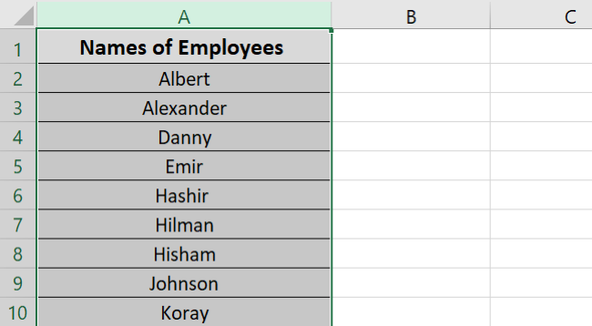
That was pretty easy, no? 😄

Let’s try something a little more difficult below.

Sort data based on multiple columns

In the following data set, we have three different column headings.

And the data is just all messed up.

Let’s fix it up. To do that:

1. Select the entire data set.
2. Click Sort.

3. The Sort dialog box appears.

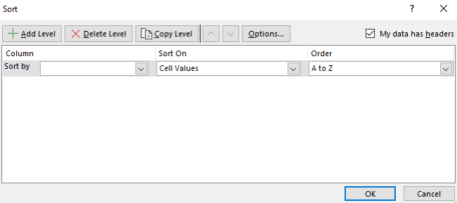
4. Under the Column heading, click the Sort by drop-down button and select a column you want to sort.

5. Then click Add level and choose the column you want to sort next.

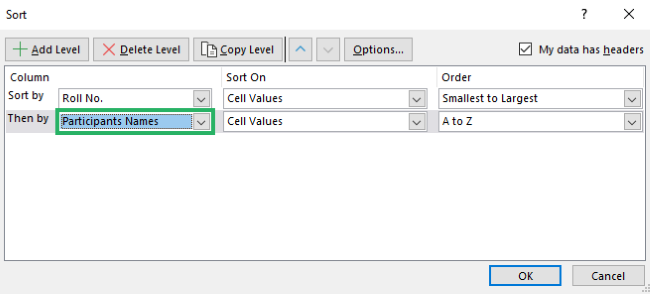
6. Make sure Sort on is set to Cell Values and Order is set to A to Z.
7. Press Enter

Excel will sort all the selected data as:

And tada! It’s done 🥳

Sort data by color

Sorting data by color is the same as sorting it by column – but only more colorful 😀

Let’s see how to sort data using colors.

Say, we have the following data.

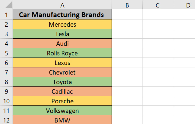
It’s pretty difficult to make any sense of this data set.

To fix it:

1. Select all the data.
2. Click the Sort button.
3. Select Cell color from the Sort option.
4. Choose the color from Order and ensure the drop-down is set to On Top.

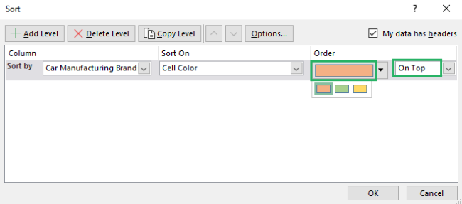
5. Add level and select the second color to sort.
6. Add another level until the Sort Options dialog box looks like this:

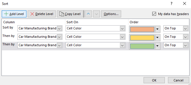
7. Press Ok.

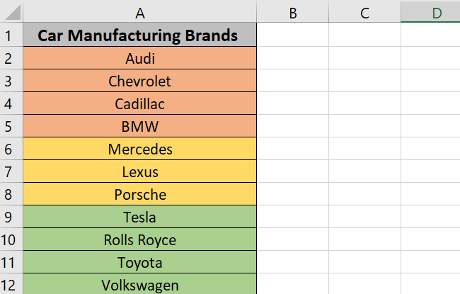
Your data is all sorted 🤗

It looks better now, doesn’t it?

Sorting with the filter button

The Sort option is great for sorting data in one go. But it can take some time to set everything up. A faster solution to this is the Filter option.

Once enabled, it appears as a drop-down button next to the column heading. And you can quickly sort data using those options.

To enable the Filter option for sorting data:

1. Select all your data
2. Go to the Data tab.
3. Click the Filter icon under the Sort & Filter group.

Alternatively, you can find it in the Editing group on Home Tab.

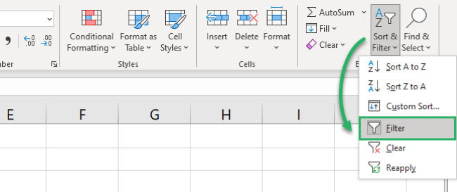
As soon as you click the Filter button, drop-down buttons appear next to each column heading. Like this:

4. Click the drop-down button, and a menu will appear.

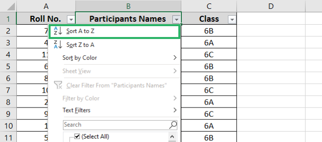
5. Select any option, and Filter will apply it to the data set.

For instance, we want to sort this data from A to Z. Just click the option Sort A to Z option, and it’s done.

Custom sorting

We’ve seen how to sort data by color and filter but what if you want to custom-sort your data?

Often we want to sort our data in an order that Excel doesn’t offer by default. That’s where the custom list comes in 😀

It lets you specify how you want to sort your data and you can create your own custom lists.

Say we have the following data.

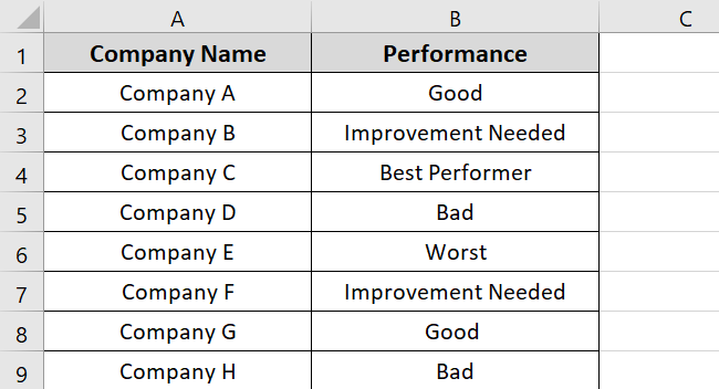
And we want to sort the performance of each company from good to bad. We cannot use the ascending or descending order in this case because the word good comes after bad.

So to sort this data, we will create a custom list.

To do that:

1. Select the data.
2. Click the Sort button – the Sort dialog box will open.
3. Select the column Performance.
4. Under the Order drop-down, select Custom list.

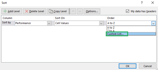
5. The Custom lists dialog box appears.

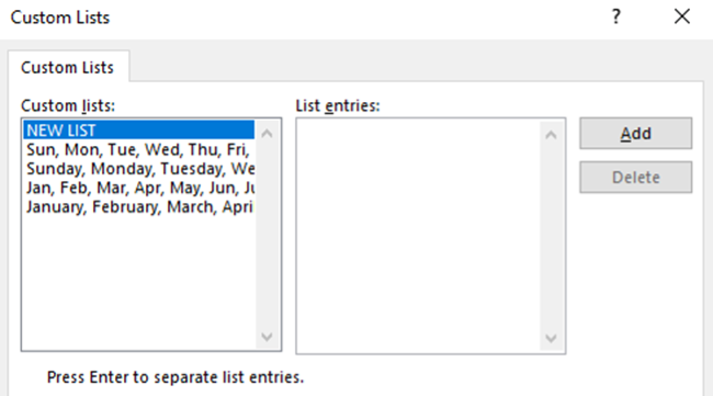
6. Add your customized list.

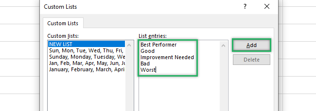
7. Press Add – the list will appear under the Custom lists heading as:

8. Press Ok.

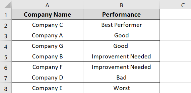
Excel has sorted all your data exactly according to the customized list entries 😊

That’s it – Now what?

In this article, we learned how to sort data by columns. We also saw how to sort data by color, using filters and even custom sort data.

Although this article explains the Excel Sort tool in detail, there is still so much to know about it. Like the special SORT function in Excel that offers advanced sorting functionality 🤓

Excel offers a plethora of other tools that you can learn to expand your skills. And in this sea of functions, it can be confusing to decide where to start.

We recommend you start out with the SUM, COUNT, and AVERAGE functions. You can learn them for free in my 30-minute email course that is delivered right to your inbox. So enroll today merely at the cost of your email address 😃

Other resources

Excel’s Sort tool is although simple, it’s great for quick sorting. It offers powerful features that can help sort data in seconds.

If you enjoyed reading this article, we’re sure you’d love to know more.

Read similar topics: Randomize a List, Conditional Formatting, Filters, and more.

Frequently asked questions