How to Calculate and do an ANOVA Test in Excel

The ANOVA test of Microsoft Excel is a great statistical tool that helps you find significant differences between two or more data groups.

Never mind if you’re hearing the word ANOVA for the first time – the word might be alien but the concept is something we need and apply in our daily lives 🚴‍♀️

To run an ANOVA test in Excel, you’d need the Data Analysis Toolpak facility which allows you to perform complex statistical analyses like a breeze. To see how to do that, grab your free practice workbook for this guide now, and come along, I will walk you through the steps to calculate and do an ANOVA test in Excel.

Table of Contents

What is ANOVA

ANOVA stands for Analysis of Variance. This statistical test of Excel is used to check if the means of three or more independent data groups are statistically and significantly different, or not.

It helps to determine if the differences between the means of these groups represent actual differences (between the means of population) or if they have occurred by chance 📝

ANOVA test is the appropriate choice to make when you want to compare the variance between three or more groups. For example, if you’re going to compare the sample data of student heights from three different schools.

There are two kinds of ANOVA tests that you can perform in Excel.

• One-way ANOVA (or One-variable ANOVA test):

The One-way ANOVA test is used when you have one independent variable within multiple groups, and you want to see if this differs from the independent variable.

For example, if we compare the test scores of students from three different Schools (Schools X, Y, and Z), the school is and independent variable, and the test scores are the dependent variable (dependent on how good each school is).

Performing a one-way ANOVA test on the sample or scores of these students will help you know if the performance of each school is significantly different from the other (analysis of variance in scores) 🏫

• Two-way ANOVA (or ANOVA: two-factor test):

The Two-way ANOVA test is to be used when you have two independent variables, and you want to test how these variables interact and cause differences to a dependent variable.

Talking of the same scores and school example above. If you want to see how three different schools (first independent variable) and their faculty (second independent variable) affect the test scores of students, you can run the 2-way ANOVA analysis 👀

One-way ANOVA test in Excel

Performing a one-way or one-variable Anova test in Excel is quite straightforward. Let me show it to you through an example here.

Here I have data on test scores from three different schools, say School X, School Y, and School Z 🎓

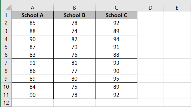
To run an analysis of variance to see if the mean of test scores from these three schools is significantly different, follow the steps below.

ANOVA test is a part of the Data Analysis Toolkit of Excel that won’t be there on your ribbon by default. To add it to the Excel ribbon:

Step 1) Go to the File tab.

Step 2) Go to Excel Options.

Step 3) From the pane on the left, click on Add-ins.

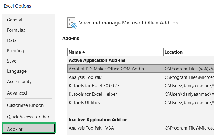
Step 4) From the bottom of the window, select Excel Add-ins and click on Go.

Step 5) Check the option for Analysis ToolPak and click Ok.

The Analysis group will be added to the Data tab 👇

Step 6) Go to the Data tab > Analysis Group > Data Analysis.

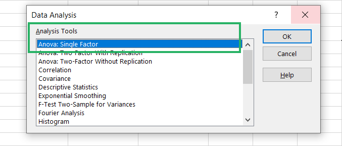
Step 7) Select Anova Single Factor and click on Okay.

Step 8) As the input range, select the data on which the ANOVA test is to be run (including the headers).

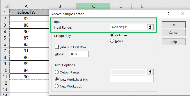
Step 9) Our data is grouped as three different columns so I am checking ‘Columns’ as Grouped By.

Step 10) Check labels in the first row as our data has labels/headers in the first row.

Step 11) The Alpha Value is set to 0.05 (we’ll let it be that for now).

Step 12) For the output range, define the cell range where you want the results of the ANOVA test populated.

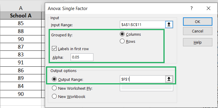
Step 13) All details are done, now click on Okay.

Excel will run the one-way ANOVA test for you and return the results as follows.

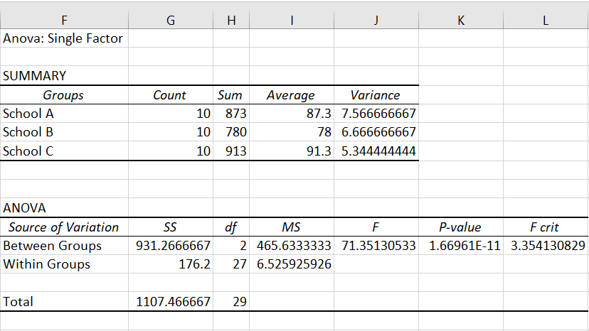
Running a one-way Anova test is this simple in Excel.

The results might seem like too much to digest now. But keep your calm, we will break them down to understand what it means in the next section 🥂

Interpreting the results of the One-way ANOVA test in Excel

Here are the ANOVA test results for the one-way ANOVA test that we ran for the test scores of three different schools above.

What do they tell you about the dataset? Let’s see that here 😎

The Summary Table

• Count: This simply counts the number of data points (test scores) in each group (school).
• Sum: The sum tells the total of all test scores in each group.
• Average: The average (mean) is calculated by dividing the sum of the test scores by the count of students.
• Variance: Variance tells how much the test scores of each school deviate from the mean. The formula for variance is the sum of squared differences between each square and the group mean.

Stats from the Summary table are easy to decode. More like some basic statistical figures for your dataset put together.

ANOVA Table

• Source of Variation: The variation in data can take two types. It can be between the different data groups and within the same data group.
• Between Groups: Between groups stats represent the variation in means of different groups due to the independent variable (as discussed above).
• SS (Sum of Squares): Before I explain to you what it represents, let me show you how is it calculated 🔎

1. Find the mean for each group which is already calculated in the Summary table as 87.3, 78, and 91.3.
2. Calculate the overall mean for all the three groups. It is 85.53.
3. Now calculate the sum of squares for each group by using the following formula:

This will give you 31.21, 567.51, and 332.54 for School A, School B, and School C, respectively.

Sum all these numbers up to get the sum of squares as 931.267.

The sum of squares is the total variation between the group means.

• Df (Degrees of Freedom): It is simply the number of groups less 1. We are analyzing three independent groups so the df is 2 (3 less 1).

The degree of freedom tells the number of independent comparisons that you can make between the groups.

This represents the number of independent comparisons you can make between the groups 👩‍🎓

• MS (Mean Square): Just like the Sum of Squares is the total variation between all three groups, the Mean Square represents the average variation between the three groups.

To calculate it, you divide the SS (Sum of Squares that is 931.467) by the df (Degrees of Freedom that is 2).

• F (F-statistic):

Let me show you the formula for the F-statistic and half the story behind it will automatically begin to make sense.

The F-statistic is a measure that compares the variance between the group means and the within the groups. The higher this number is, the more these means are significantly different.

• P-value:

The P-value comes from the F-distribution table based on the F-statistic and the df 👩‍🏫

The P-value is indicative of the probability of the null hypothesis (that the means of all the groups is the same) being true. A P-value equal to or less than 0.05 rejects the null hypothesis. This might mean that at least one of the groups’ mean is significantly different.

• F crit (F critical value):

F-crit is the critical value from the F-distribution table for a given level of significance (that we have and is usually set as 5%) and the degrees of freedom 💹

The same calculations (based on the same sense) continue within groups.

Bottom Line for our ANOVA test

For the ANOVA test we’ve just run above, we have the following key stats.

• F-value: 71.35
• P-value: 1.66961E-11 (which is approximately 0.0000000000167)
• F critical value (F crit): 3.354131

Since the P-value is way smaller than 0.05 (it’s not even 0.01), we can safely reject the null hypothesis to be true (that all the group means are the same).

Talking of the F-value, 71.35 is significantly greater than 3.354 which further tells that the group means are significantly different from each other 🚀

This ANOVA results show that the mean test scores for students from all three schools, X, Y, and Z are very different. The independent variable (schools) makes a great difference to the dependent variable (test scores).

That is how the ANOVA table helps hypothesis testing and summarizes and pictures the total variability in the given datasets. It shows variability between different groups and within groups.

Conclusion

Following this step-by-step guide, you can run one-way ANOVA tests in Excel like a pro. ANOVA tests help you determine if the differences in the means of three or more independent groups are significant, or not 💪

Running an ANOVA test in Excel might not be as big of a challenge as is to interpret the results of this test. Rightly understanding the results of the ANOA test such as the P-value and F-statistic in its right sense will help you make informed decisions based on the results of your data.

We have covered all of this knowledge in the guide above. Hope you enjoyed reading this guide and if you did, do not forget to check out other similar Excel tutorials by Spreadsheeto here.

• How to Add Line of Best Fit in Excel (Easy Method)
• How to Find Coefficient of Variation in Excel
• How to Perform Linear Interpolation in Excel (Easy)