How to Use the CHOOSE Function in Excel + Examples
Just like the INDEX function, the CHOOSE function of Excel may not be very useful in itself.
But when you combine it with other functions (and the right other functions) you’ll be amazed to see how it works 😎
So let’s take you on this journey of amazement. The guide below is all set to teach you how to use the CHOOSE function in Excel.
Dive right in and click here to download our sample workbook for this guide here 📩
Table of Contents
How to use the CHOOSE function
The CHOOSE function returns a value from an array based on its position.
In simpler words, you supply an array to Excel along with the position of the value to be returned from it 🥇
The CHOOSE function is available in almost all versions of Excel starting from Excel 2007 and all versions onwards.
The syntax of the CHOOSE function has only two arguments:
= CHOOSE (Index_num, value1, [value2],…)
- Index_num: This is the position of the value to be returned.
- Value1: These are the values supplied to Excel from which a value is returned. The first value is required. Other values are optional and can be omitted.
Pro Tip!
The CHOOSE function can only process up to 254 values. These can be numbers, cell references, text values, or other formulas 🎯
Enough of the talking! Let’s now see an example of the CHOOSE function in action 🚴♂️
So here’s a list of names in Excel.
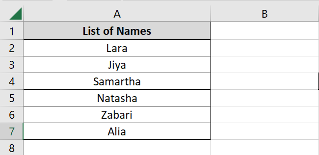
Let’s write the CHOOSE function to extract the third name from this list.
- Begin writing the CHOOSE function.
= CHOOSE (
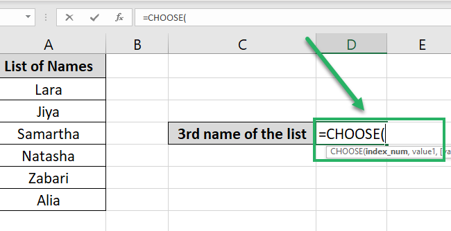
- Write 3 as the index_num 3️⃣
The first argument is the index number. This is the position of the value that you want to be returned. As we want the third value from this list, we are setting it to 3.
= CHOOSE (3,

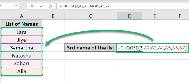
- Refer to each cell of the list containing the values.
= CHOOSE (3, A2, A3, A4, A5, A6, A7)
Pro Tip!
You cannot specify the entire cell range A2:A7 as the value argument. Doing so will result in the #VALUE error ❌
Excel will consider the range A2:A7 as a single value. With one value supplied, you cannot expect the CHOOSE function to return the 3rd value. As it fails to find any 3rd value, it returns the #VALUE error.
- Hit Enter to see the results.
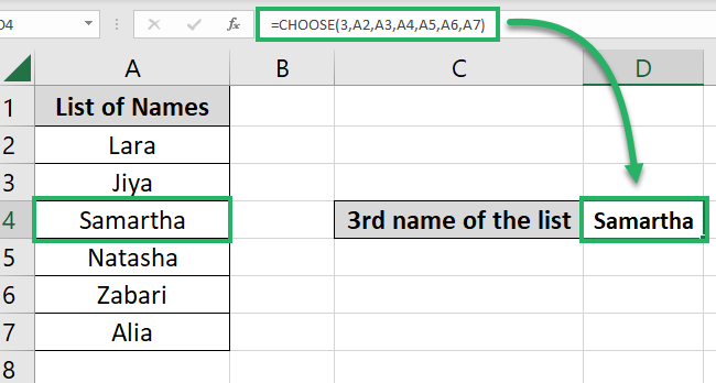
Samartha is third on the list 🥉
The CHOOSE function is one of the simplest functions of Excel. And if you are thinking why anyone would even want to use such a basic function – you are 200% on point 🤔
The examples below will answer your question.
Other CHOOSE formula examples
Hold on tight! We are now moving into the sections of CHOOSE function examples that will have you amazed.
CHOOSE example #1: VLOOKUP/CHOOSE: Left lookup
If you’ve ever used the VLOOKUP function, you’d know the one and the biggest flaw of this lookup function 💁♀️
Yes – you guessed that right. The VLOOKUP function can only fetch values from the right side of the table array.
And what if you have to perform a left lookup? 👈
The simple VLOOKUP function would fail there. But if you nest the CHOOSE function inside the VLOOKUP, you’re all sorted. See that here:
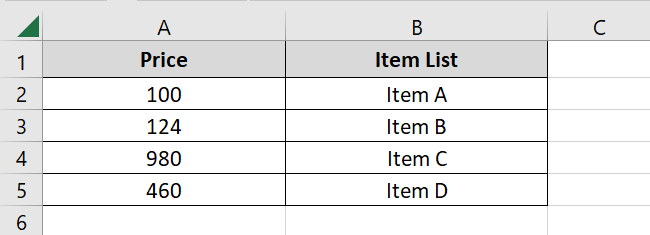
The data above has a list of items with their prices mentioned to the left. Using the item name, can we fetch the price for each product?
- Write the CHOOSE function as follows:
= CHOOSE ( , B2:B5, A2:A5)
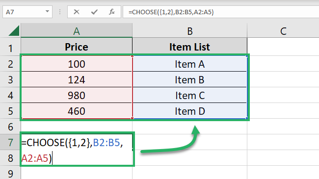
- Hit Enter, and you’d see these results.
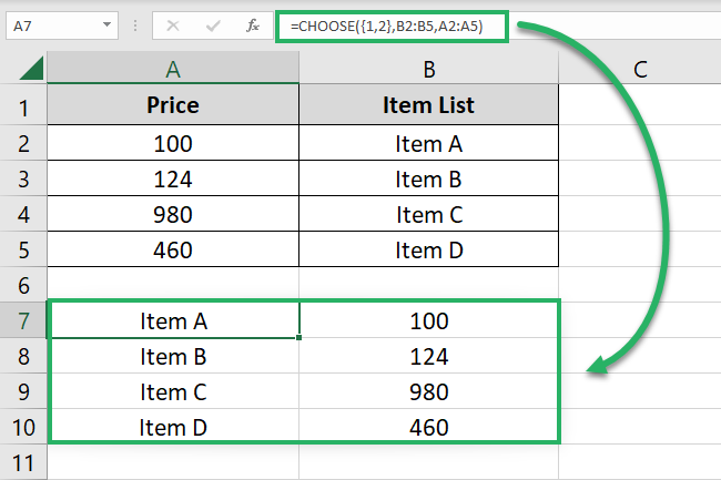
What just happened? We supplied two index numbers to the CHOOSE function.
As Value1, we supplied the range B2:B5, and as Value2, we supplied the range A2:A5. So the CHOOSE function returned both the values (ranges) but changed their positions.
So now range B2:B5 (Item names) becomes Column 1, and range A2:A5 (prices) becomes Column. Problem solved 💪
- Now write the VLOOKUP function as follows:
= VLOOKUP (“Item A”,
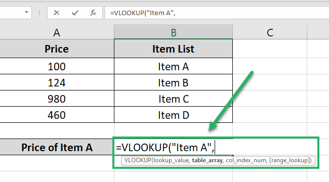
- Nest the CHOOSE function (as above) as the table array of the VLOOKUP.
=VLOOKUP("Item A",CHOOSE(,B2:B5,A2:A5)
- Specify 2 as the column number from where the value is to be fetched.
Prices have now become column 2 in the table array referred to above, so our column index number will be 2.
=VLOOKUP("Item A",CHOOSE(,B2:B5,A2:A5),2)
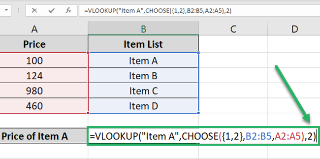
- Hit Enter, and there you go!
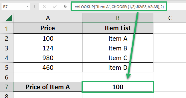
The answer is 100 – the price for Item A which is correct 🚀
Hope you enjoyed this!
CHOOSE example #2: Replacing Nested IF functions
The image below shows the performance of 4 different companies in terms of percentage points 🎭
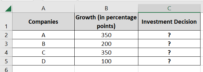
A company that has 200 percentage points to its credit has grown in value by 20%, and so on.
So is that good of a performance for a Company or not? The performance key below will tell that 👇
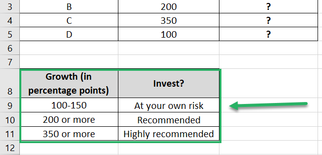
Based on this performance key, which company should we invest in it? To populate the column for investment decisions, you’d ordinarily write the IF function as below.
=IF(B2>=350, “Highly Recommended”, IF(B2>=200, “Recommended”, IF(B2>=100, “At your own risk”, “Not Recommended”)))
This means you’re telling the IF function to return:
- “Highly Recommended” if the performance score is more than or equal to 350 points.
- “Recommended” if the performance score is more than or equal to 200 points.
- “Invest at your own risk” if the performance score is more than or equal to 100 points.
- “Not Recommended” if the performance score is less than 100 points.
Now let’s try doing the same using CHOOSE function 🎲
- Write the CHOOSE function as follows:
= CHOOSE ( (B2=>100) + (B2=>200) + (B2>=350), $B$9, $B$10, $B$11)
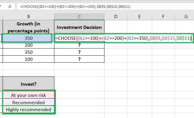
As the index number, write the performance scores as logical conditions starting with the smallest (equal to or greater than 100).
For the value argument, list all the cells containing recommendations in ascending order. This means the lowest grade recommendation (Invest at your own risk) comes first, and so on ✍
Pro Tip!
If Cell B2 is equal to 350, the expressions B2>100, B2=>200, and B2=>350 will return TRUE.
For most of the Excel functions, TRUE is equal to 1, and FALSE is equal to 0.
So the above function would become:
= CHOOSE ( 1+1+1, $B$9, $B$10, $B$11)
Which means:
= CHOOSE (3, $B$9, $B$10, $B$11)
And the CHOOSE function would return the 3rd value (B11) from the cells referred to above. Cell B11 contains Highly Recommended, and that’s what we know is the right answer ✅
Similarly, for Cell B4 (that contains 100), this function becomes:
= CHOOSE (1+0+0, $B$9, $B$10, $B$11)
And the CHOOSE function returns Cell B9 (the first value) that says “Invest at your own risk”.
- Hit Enter to get the results as follows:
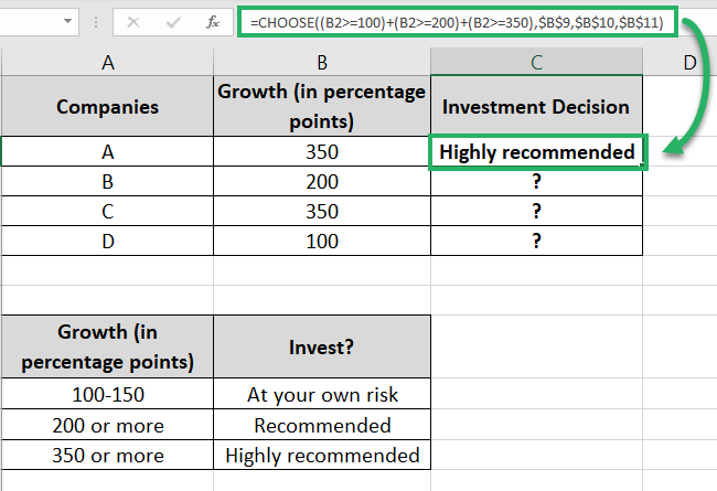
Just like expected. The CHOOSE function extracts the correct recommendation for the given performance score ✌
- Drag and drop the results to the whole list.
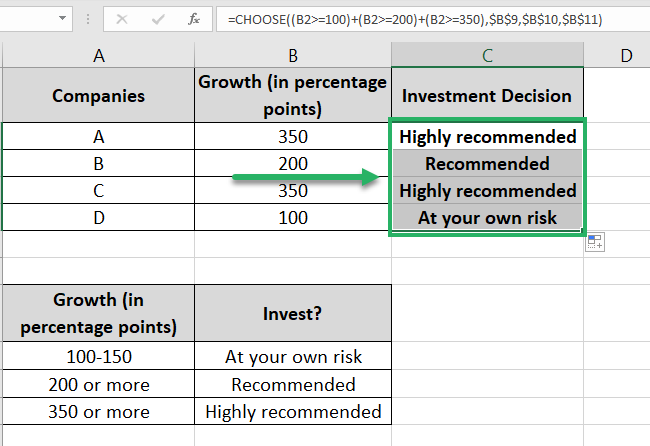
Note that we have turned the cell references for the value argument into absolute references 💲
This is to prevent the automatic changing of cell references when the formula is dragged and dropped across other cells.
That’s how you can use the CHOOSE function to replace the long and complex nested IF function. 🕸
Interesting, no?
That’s it – Now what?
The above guide comprehensively teaches how to use the CHOOSE function in Microsoft Excel.
Starting from its syntax to multiple examples of how you can use it together with other functions – we have learned it all 🏆
The CHOOSE function can prove super useful when used together with the relevant Excel functions. There are just so of them for you to explore.
Some of my top favorite functions from Excel include the VLOOKUP, SUMIF, and IF functions. Easy to use but very useful.
Other resources
The Excel CHOOSE function works just like the INDEX and MATCH functions do. Want to see how they work?
