How to Fix the #Value Error in Excel (Step-by-Step)

If you are an Excel user (even if a newbie), you must have come across the #VALUE error of Excel ⚡

It looks very distasteful and alarms the whole sheet.

When does the #VALUE error occur and how can you fix it in Excel? If you are on the hunt to find the answers to these questions, you are in the right place ✔

Continue reading the guide below to learn all about the #VALUE error in excel.

And while you scroll down, download our sample workbook here to tag along with the guide.

What causes the #VALUE error

The first step towards solving any problem involves diagnosing the problem. So what causes the #VALUE error?

Through the #VALUE error, Excel is saying that there is something wrong:

• With how the formula is typed.
• Or with the cell reference.

The exact reasons why the #VALUE error occurs depend upon the formula being used 🔍 However, here are some general reasons why the #VALUE error may occur:

Wrong Data Type

If you are specifying the wrong data type for any given formula, you’ll likely end up having a #VALUE error.

For example, here:

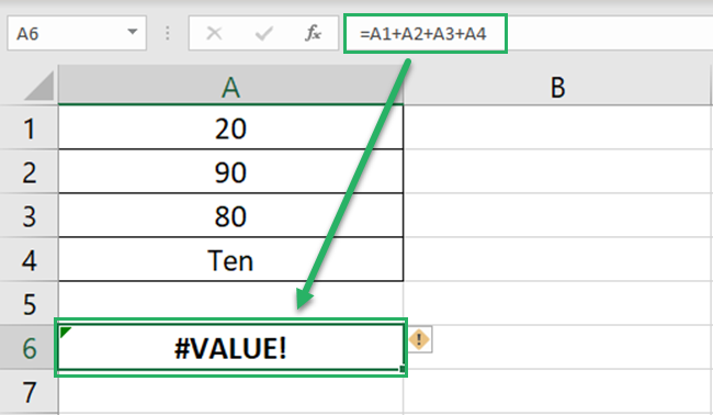
Excel can surely sum up numbers but not text. As the list contains the text “ten”, the formula to add the cells returns a #VALUE error.

Had we used the SUM function here instead of operators, the result would have been different. Why? We will see that soon 🤔

Wrong Cell references:

You’d often see this happen when you drag and drop the formula to a whole list. Check this out here:

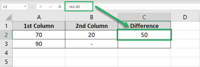
The first formula is to subtract two cells. And the result is accurate 🎯

However, when the same formula is dragged and dropped to all the cells, the answer is a #VALUE error.

This is because one of the cells for the second formula doesn’t have the right value.

Cell B2 contains a dash (-). And Excel can certainly not deduct a dash (-) from 10, so we get the #VALUE error.

Incorrect Function arguments

Whenever you end up with a #VALUE error, double-check your function for accuracy. More precisely, check it logically.

For example, the FIND function of Excel finds the position of a character from a text string.

The formula FIND (“a”, “dark”) gives the result 2. Because the substring “a” comes in the second position in the word “dark” 2️⃣

Now try writing this formula as below:

=FIND (“j”, “dark”)

And Excel returns a #VALUE error.

That’s because the word “dark” just doesn’t contain the character “j”, let alone its position therein.

How to fix the #VALUE error

We know the common problems that may potentially cause the #VALUE error. Now is the time to seek the solution to these problems.

To fix the #VALUE error, try out the hacks below 👇

Check for any special characters:

Check out your data for any non-numbers or texts, or other characters. These might be space characters or other special characters.

You cannot differentiate between space characters and blank cells in Excel. But you can use the ISTEXT function to identify them. See below:

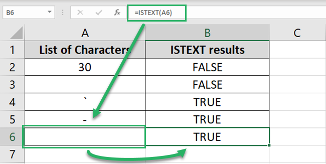
Cell A1 is apparently empty but contains a space character. The ISTEXT function gives the result TRUE (Yes, this cell contains some value) 👀

Once you have identified the cells that contain space characters, clear them out. Then try running your formulas and you’ll likely steer clear of the #VALUE error from your spreadsheet.

Use Excel functions instead of operators

Use in-built functions of Excel instead of writing formulas using operators. Functions in Excel are usually developed to ignore any non-text value.

Check out here:

Cell B2 here consists of a dash (-) and is not empty.

Now write the following formula:

= A2 * B2

We have a #VALUE error as Excel cannot multiply 25 with a dash (-) 🙅‍♀️

Now write the PRODUCT function for the same:

= PRODUCT(A2,B2)

The PRODUCT function returns 25 but not a #VALUE error.

Double-check the format of your data.

For example, in the image below, we have applied the WEEKDAY function that returns the day for any given date.

But the function gives a #VALUE error. This is because Cell A1 contains the date in a general format. And that is not a valid date for the WEEKDAY function.

Change the format to date.

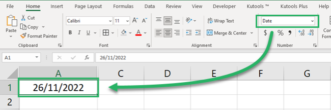
And now retry applying the WEEKDAY function:

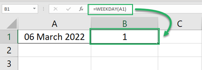
Yay! No more #VALUE errors 🏆

Replace the #VALUE error

Sometimes, you know a #VALUE error would occur. And the problem is not with Excel returning an error.

The problem is with the #VALUE making a distasteful appearance on your worksheet.

If that’s the case, you can simply replace it using the IFERROR function. For example, the function below returns a #VALUE error.

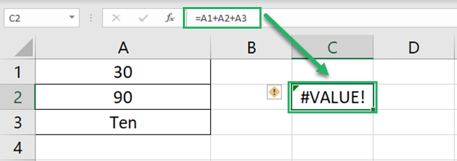
Simply wrap it in the IFERROR function as follows 🎁

= IFERROR ((A1+A2+A3), “-“)

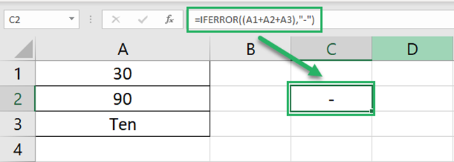
The IFERROR function will replace #VALUE with a dash (-). You can specify and value instead of a dash, as desired.

Evaluate the Formula

This is the last resort – when you have tried everything else but have still not found the cause of the error.

In such a case, let Excel evaluate the formula and spot the cause.

Select your formula (that returns a #VALUE error). And go to the Formulas Tab > Evaluate Formula.

Excel would evaluate the formula and tell you what’s causing the error.

For example, Excel tells that 30 and 90 are added up to make 120. But in the next step, it’s the text causing the error here.

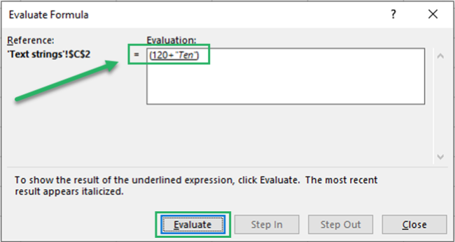
Remove the cause of the error as identified by Excel. And rerun the formula to see if it works.

Examples of formulas that return the #VALUE error

Very honestly, the list of formulas that return the #VALUE error might be too long to list here.

That’s because most of the formulas in Excel (that are not rightly fed or structured) will give the #VALUE error.

So, let’s see a few examples of these formulas:

Example No. 1: SUMPRODUCT Function

The SUMPRODUCT function multiplies two (or more) arrays with each other. And then adds up their product.

Let’s write it as follows:

= SUMPRODUCT (A2:A4, B2:B3)

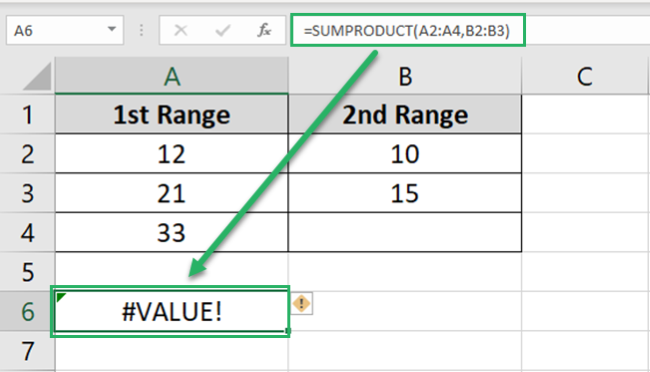
And guess what! We end up having a #VALUE error.

Why? Hard to note, but we have made a very logical mistake. The first range has three cells (A2 to A4).

Whereas the second range has only two of them (B2 and B3) 😵

Excel will multiply Cell A2 to B2, Cell A3 to B3, and for Cell A4, there is no other cell. This causes the #VALUE error.

Add another cell to the second range (make it B2:B4 from B2:B3). And reapply the SUMPRODUCT function:

= SUMPRODUCT (A2:A4, B2:B4)

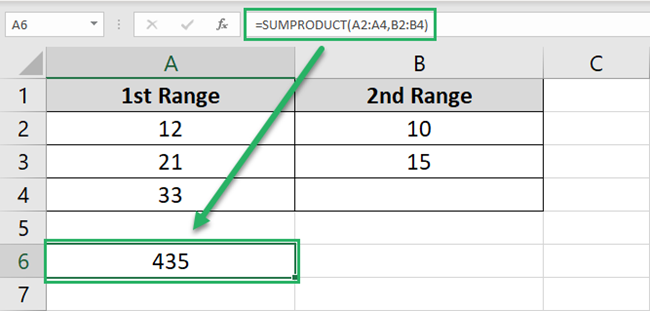
Excel now has all the cells in place to apply the SUMPRODUCT function. And though cell B4 is empty – the SUMPRODUCT function doesn’t return the #VALUE error ✌

Example No. 2: DATE function

Do you know that Excel treats each date as a serial number?

Where 01/01/1900 is equal to 1, 02/01/1900 is 2, 03/01/1900 is 3, and so on.

So what number is 30/05/2022? Don’t go on counting manually – it will take you hours or maybe days to reach the answer ⏳

Instead, write the DATE function as follows:

= DATE (C2, B2, A2)

Cell A2 contains the date, B2 contains the month, and C2 contains the year

But Excel returns a #VALUE error.

That’s because the month is in “text” format. Excel only recognizes it in numbers.

Change the month to number format and reapply the DATE function now:

= DATE (C2, B2, A2)

30th May 2022 stands at serial number 44711 🚀

That’s it – Now what

We have had a super detailed discussion on the #VALUE error of Excel in the guide above.

From diagnosing the problem that causes the #VALUE error to solving it – we have seen it all.

Let’s not forget the list of functions that return the #VALUE error when applied the wrong way. You might have found this list short but let me burst your bubble💭

The library of Excel functions is way too vast. And if you want to start learning these already, I suggest you begin with the VLOOKUP, SUMIF, and IF functions.

These are some basic, yet very useful functions of Excel. To get your hands on them, enroll in my 30-minute free email course today!

Other resources

Taking a smarter approach, you can identify erroneous formulas beforehand by using the ISERROR function.

Or you can identify error values and replace them with any value of your choice by using the IFERROR function.

Learn how to use the ISERROR and IFERROR functions of Excel here.

Frequently asked questions