How to calculate a correlation coefficient in Excel
When we do data analysis, we usually check 2 things about variables.
- What is the strength between them? (strongly correlated or not )
- What is the pattern between them? (the variable x increases or decreases with the change in variable y)
To check that, we have to do a correlation analysis.
This is the formula to calculate the Pearson correlation coefficient😱

The above formula is too complex to calculate the correlation coefficient.
You have to do many complex calculations to get the final answer. Isn’t it a headache for you?🙄
Relax! Excel will take care of all your problems🤔
The Correlation Coefficient can be quickly calculated in Excel. Just need to select two columns with data points for the formula😊
You can use Excel’s “Data analysis Tool Pak” if you wish to compare more than two variables in your data analysis👍
I’ll explain how to do correlation calculation functions in Excel using the below data set.
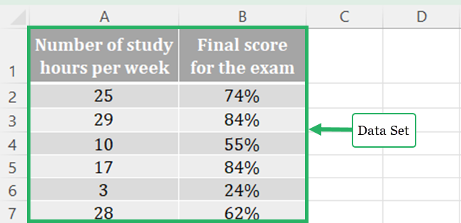
If you want to follow along with me, you may click here to get the practice workbook.
Before we start, let’s go over some important points about correlation coefficient values.
- Correlation coefficient values range between -1 and +1.
- When there is a positive correlation coefficient, both the x and y values increase.
- If there is a negative correlation coefficient, x increases when y decreases or x decreases when y increases.
- If the correlation coefficient is +1, two variables have a perfect positive correlation.
- If the correlation coefficient is -1, two variables have a perfect negative correlation.
- Variables are strongly correlated when the correlation coefficients are near +1 or -1. If it is near zero, the correlation coefficient is weak.
Table of Contents
Calculating the correlation coefficient with the CORREL function
Let’s see how to calculate the correlation coefficient in Microsoft Excel.
In our data set the dependent variable (variable y) is the final score, and the independent variable (Variable x) is the number of study hours. Because the final score is affected by the number of study hours.
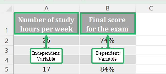
Identifying the independent and the dependent variable is not important for the correlation. We can interchange x and y in the correlation coefficient formula.
- Enter an equal sign and choose the CORREL function.
Write:
=CORREL(
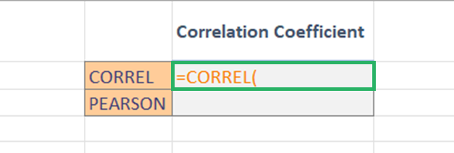
- As array 1 of the above formula, select a data range of one variable.
As array 1, I select all data points from the number of study hours.

Now your formula is:
=CORREL(A2:A17
- Select the data range from the second range as array 2.
I select data from the final score column for array 2 of the correlation formula.

Your formula should look like this by now:
=CORREL(A2:A17,B2:B17)
- Zero values are included to calculate the correlation coefficient in Excel.
- Text, logical values, and empty cells are not included to calculate the correlation coefficient in Excel.
The correlation value for our data set is ready.😊
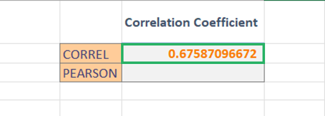
For the correlation coefficient, Excel calculated a value of 0.68.
It indicates that there is a strong positive correlation between the 2 variables.
Pro Tip!
Is there a #N/A error for the correlation coefficient in Excel? It says that 2 variables in your data set have a different number of points.
Is there a #Div/0! error for correlation coefficient in Excel? It says that the data set of either one variable is empty, or the standard deviation of their values equals zero.
It is now clear that calculating the correlation coefficient in Excel is both easy and fast! 👍
Calculating correlation coefficients with Data Analysis
Do you want to calculate the correlation coefficients of a data set that has more than 2 variables?
You can’t use the CORREL function as it allows only 2 variables.
No problem! You can use the data analysis toolpak option in Excel.
It will create a correlation matrix. You can see all correlation coefficients between each pair of variables at once.
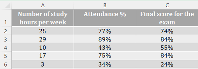
Let’s apply it to the below data set.
- Go to the “Data” tab.

- Go to the “Data analysis” icon in the “Analysis” section.

Pro Tip!
If the “Data analysis” icon is not visible, you have to load the analysis toolpak.
- Go to the “File” tab.

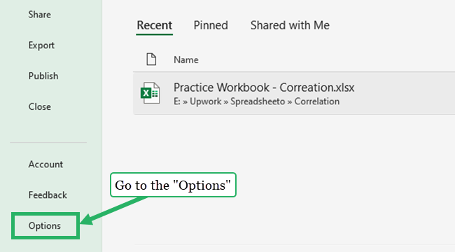
- Go to the “Options”
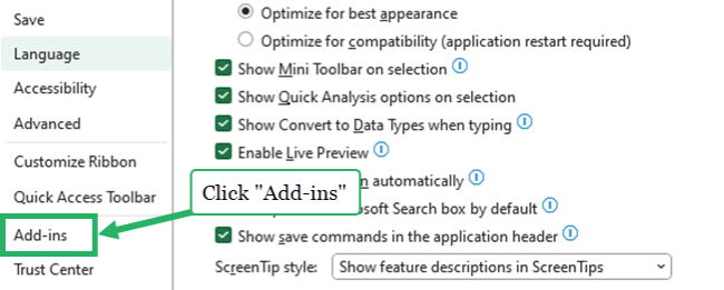
- Click on Excel “add-ins” category from the Excel options dialog box.
- Click “Go” in add-ins.
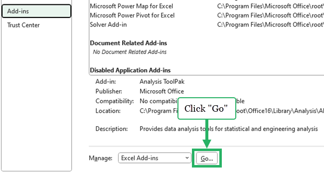
- Check the Analysis ToolPak checkbox in the Add-Ins box, and then click OK.

- Click the “Data analysis” icon to open the data analysis dialog box. Then, select “correlation” from the list.
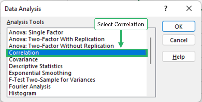
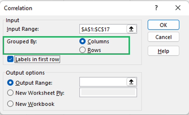
- Now you have to enter input and output options in the correlation dialog box.
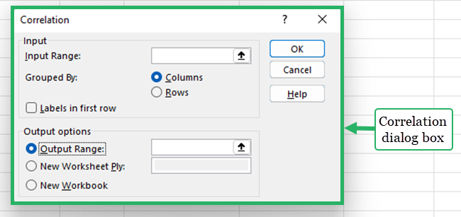
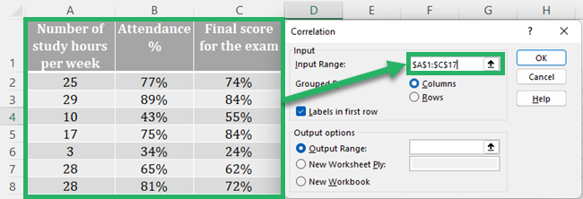
First, select the input range. I select the entire data table range including headings.
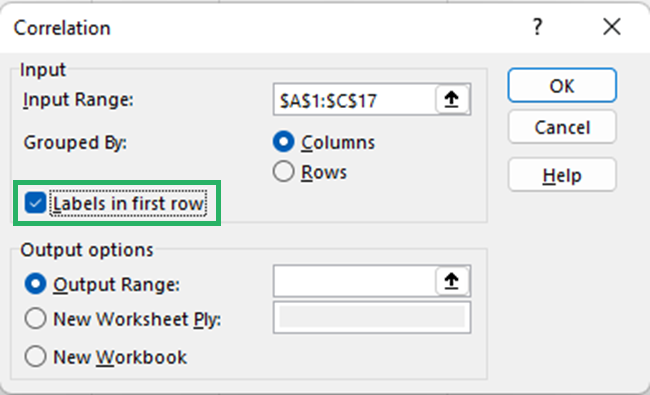
As I selected the input range with the headings, I check “labels in first row”.
Select data set is grouped by columns or rows. As our data set is grouped by columns, I select “Columns”.
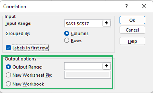
Next, select one of the output options.
- If you want the output table or Excel correlation matrix in the same Excel worksheet, select “Output range” and specify the range.
- If you want the Excel correlation matrix in a new worksheet in the same Excel workbook, select “New Worksheet Ply” and give a name to that worksheet.
- If you want the correlation matrix in a new Excel workbook, select “New Workbook”.
I want to get the output table in the same Excel sheet, So I select “Output range” and select the cell “E1”.
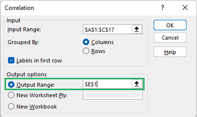
- Click “OK” to get the Correlation matrix.
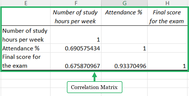
From the table, we can see below correlation coefficients.
- Number of study hours and attendance %: 0.690575433806873 (Positive)
- Number of study hours and Final score: 0.675870966721747 (Positive)
- Final score and attendance %: 0.933704960358332 (Positive)
Calculating the correlation coefficient with the PEARSON function
Excel has another function called “PEARSON” to calculate the Pearson correlation coefficient.
- Enter an equal sign and choose the PEARSON function.
Write:
=PEARSON(
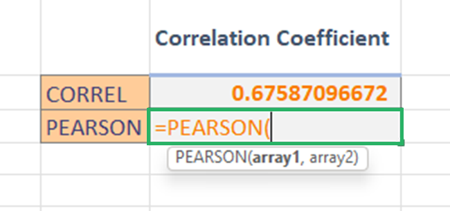
- As array 1, select the set of independent values.

Now your formula is:
=PEARSON(A2:A17
- As array 2, select the set of dependent values.

Pearson’s correlation coefficient in Excel is ready!😊
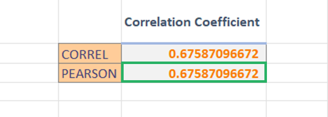
Your formula should look like this by now:
=PEARSON(A2:A17,B2:B17)
Except for Excel versions earlier than Excel 2003, the “PEARSON” function’s result is the same as the “CORREL” function’s result in every case.
Pro Tip!
Use the “CORREL” function if you are using an Excel version earlier than Excel 2003. Because the PEARSON function has rounding errors in earlier Excel versions.
That’s it – Now what?
Now you know that it is super easy to find correlation coefficients using Excel.
Do you know that you can use VBA Excel to create your own macros that can perform any statistical functions?
Sounds interesting?😍
To learn macros, start our free Excel Advanced user training: “Mighty Macros“.
Other resources
Would you like to get an overview of the analysis toolpak?
Then read my step-by-step guide to it here.
Also, don’t forget to read our article about Linear Regression too.
