How to Find Duplicates in Excel Using a Formula
It’s normal to find duplicate data in your Excel files.
When you’re dealing with a small group of data, finding duplicates should be easy-peasy. But when your Excel sheet is filled with rows and columns of data, it could be stressful. 😫
Duplicate data also makes your information more confusing and difficult to assess accurately. Excel users usually find duplicates to remove them.
Amazingly, Microsoft Excel has features and formulas that you can use to find duplicates in your worksheet. 🔍
In this article, we’ll show you how to find duplicates in Excel (and with the use of a formula).
Download this sample workbook to follow along with this Excel tutorial.
Highlight Duplicates using Conditional Formatting
One of the ways to find and highlight duplicates in Excel is by using Conditional Formatting.
Conditional formatting makes it easy to highlight certain values or make particular cells easy to identify. This changes the appearance of a cell range based on a condition (or criteria).
Open your sample Excel workbook and let’s use conditional formatting to find duplicate cells in our worksheet.
Step 1) Select the cells that you want to check for duplicates.
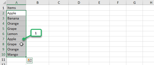
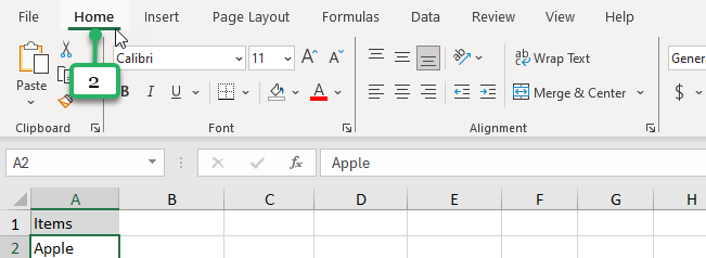
Step 2) Go to the Home Tab.
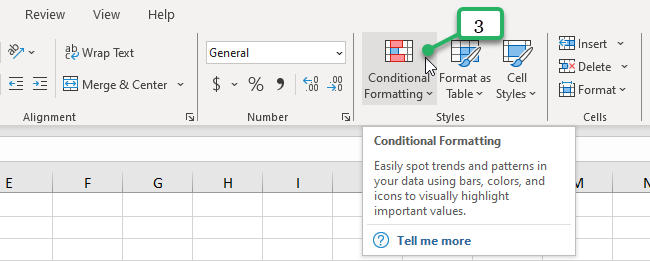
Step 3) In the Styles group, click Conditional Formatting and a drop-down will appear.
Step 4) When the drop-down menu appears, hover your cursor over the Highlight Cells Rules option and it will show another menu.
Step 5) Click the Duplicate Values option.
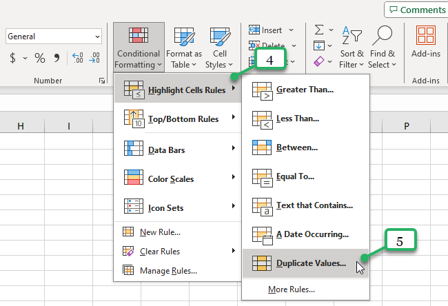
A Duplicate Values dialog box will appear.
Step 6) Select how you want the duplicate values will appear by clicking the drop-down arrow.
Step 7) Click OK.
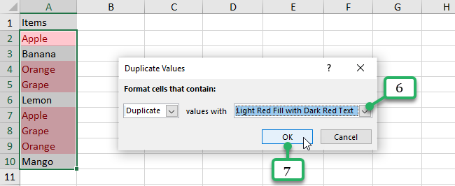
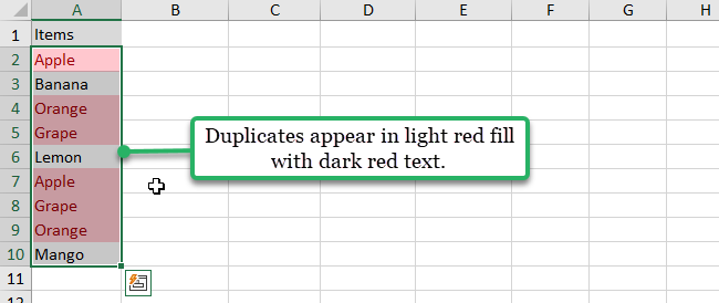
The steps above highlight duplicates in your item list. In our sample worksheet, duplicate values appear in light red fill with dark red text. 🔍
Find Duplicates using the COUNTIF Function
Another way to find duplicate values in your data set is by using the COUNTIF Function.
The COUNTIF function is one of the statistical functions that counts the number of cells that meet a criterion;
In its simplest form, COUNTIF says:
=COUNTIF(Where do you want to look?, What do you want to look for?)
The syntax of this function is =COUNTIF(range, criteria) with the following arguments:
- range (required) – the range of cells you want to count. Range can contain numbers, arrays, a named range, or references that contain numbers. The blank and text values are ignored.
- criteria (required) – a number, expression, cell reference, or text string that determines which cells will be counted.
You can use the COUNTIF function to find duplicates including or excluding the first occurrences. We will show you how in the next sections. 👇
Including 1st occurrences
In our sample workbook, let’s use the COUNTIF function to find duplicates in the list of items in column A.
To start,
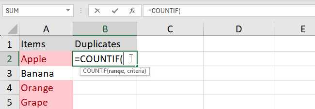
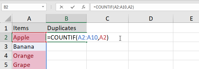
Step 1) Double-click cell B2 and type
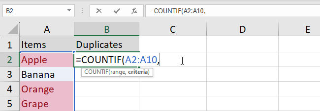
Step 2) For the range, select the cells A2 to A10. This is the range of cells you want to count. Then, type a comma symbol (,)
Step 3) For the criteria, select the first cell (Cell A2) which contains the text “Apple”, a cell value we want to find any duplicates. Then close the formula with a right parenthesis.
Step 4) Type a greater than symbol (>) and type 1.
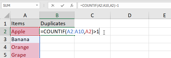
Step 5) Press Enter.
Fill in the rest of the cells by double-clicking or dragging down the Fill Handle.
As you can see, the COUNTIF formula returns TRUE for duplicate values and FALSE for unique values. 👍
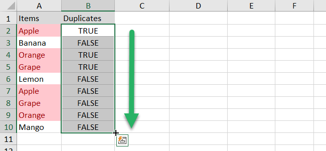
Note that using this formula doesn’t result the cells below as duplicates. That is why the COUNTIF formula above is not good to use. 😬
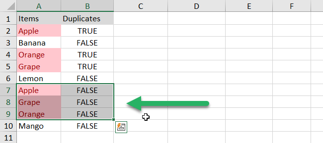
When selecting a range of cells in Excel, it’s important to lock the range of cells with the dollar ($) sign. This fixes the reference to a given cell so that it remains unchanged no matter where the formula moves.
In the steps done above, it’s better to use this formula:
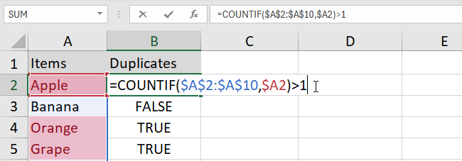
This shows correct results.
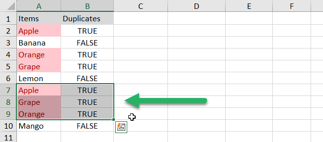
The above example shows how important relative and absolute cell references are. Click this article to learn more about how important is the dollar sign ($) and how to use it in your Excel formulas.💡
You can make the duplicate formula into something more clear and meaningful than the Boolean values of TRUE and FALSE.
For this, utilize another function, the IF function.
You can enclose the duplicate formula we’ve used above and type the labels you want for duplicate and unique values.
For example, the formula returns “Duplicate” for duplicate values and “Unique” for unique values. You can copy this formula below:
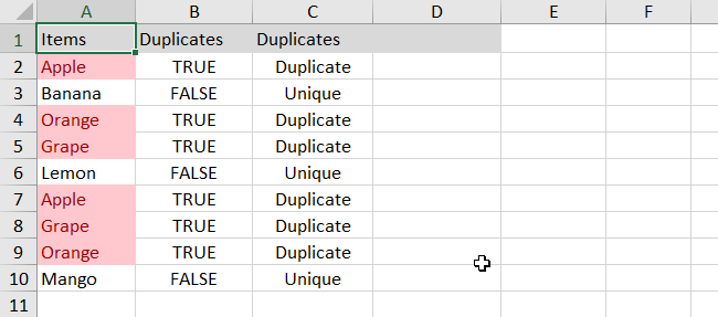
This makes it more clear. 👍
In case, you want an Excel formula to only find duplicates, replace “Unique” with an empty string (“”) like this, use this formula.
The formula will return “Duplicates” for duplicate records, and a blank cell for unique records.
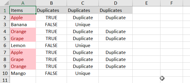
Excluding 1st occurrences
Notice that the first occurrence of “Apples” in our list is a duplicate. 👀
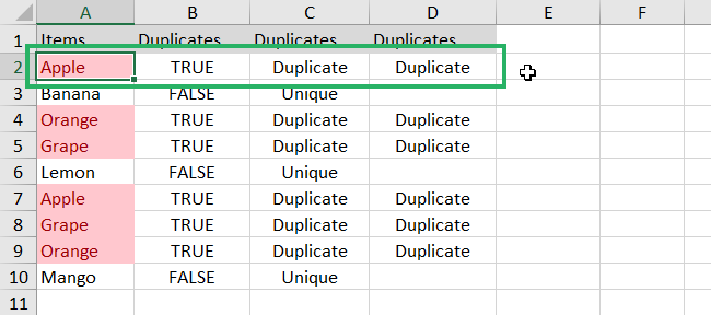
This is because using the above formula marks all the identical records as duplicates. If you decide to remove duplicates by then, you may lose some of the unique data in the process.
To avoid this, you must exclude the first occurrences and only delete the 2nd and other subsequent instances. 😊
Let’s try to use this formula:
and press Enter.
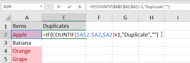
Then double-click or drag down the fill handle to fill in the rest of the cells.
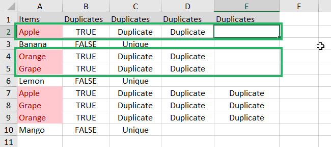
Now, the first occurrences of the items aren’t identified as duplicates. Only the second occurrences are.
That’s It—Now What?
Awesome!
Finding duplicates shouldn’t be stressful at all. With Microsoft Excel’s features and formulas, you can do this easily and quickly.
What else can Microsoft Excel do for you? Check out these related articles we’ve picked for your next read: 📚
