Use This Excel Formula to Remove Duplicates (Fast)

If you’ve ever had to deal with duplicate values in your Excel worksheet, you would know how very troublesome they can be to manage.

You can manually find and delete duplicate values when the worksheet is small but if the data is large, deleting duplicate entries can be very difficult ☹

Luckily, Microsoft Excel offers different ways how you can remove duplicate values – the quickest of which is using formulas. We will explain these methods in detail below.

Download our sample workbook here to learn how to remove duplicates in real-time. Let’s now get right into the tutorial below 🔽

Table of Contents

Remove Duplicates in Excel Using the UNIQUE Function

The UNIQUE Function offers the easiest and quickest way to remove duplicate rows in Excel. All you need to do is put in a formula and select the range and it’s done.

Don’t believe us? See for yourself below 🧐

The syntax of the UNIQUE function is :

Say, we have the following sample data set.

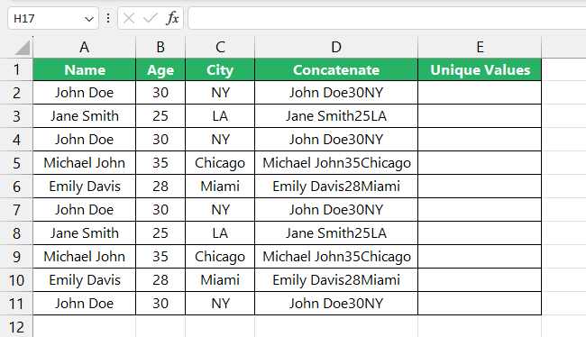
To remove the duplicate cells in the data,

Step 1) Select cell E2.

Step 2) Type in the UNIQUE formula as:

Step 3) Press Enter.

Excel will copy the formula down to the remaining cells automatically.

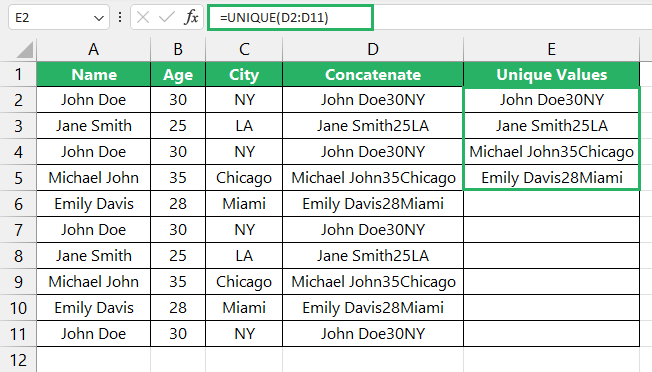
And it’s done. In two clicks, the Unique function was able to return the duplicate values in our range of cells.

How fast is that? 😃

Remove Duplicates in Excel Using the CONCATENATE Function

Another slightly longer method of removing duplicate entries from your data set using the CONCATENATE function.

Its syntax is given below.

Let’s see how to implement it below.

Say, we have the following sample data 🧾

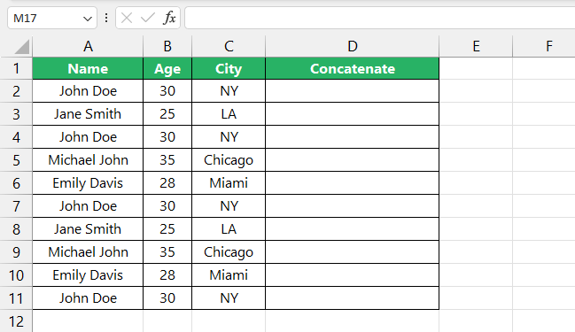
To delete duplicate rows from the data,

Step 1) Select cell D2.

Step 2) Type in the following formula in the cell:

Step 3) Press Enter.

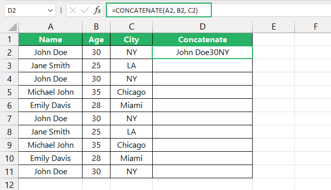
Step 4) Double-click Fill Handle to copy the formula to the remaining cells.

This is what your data set will look like now:

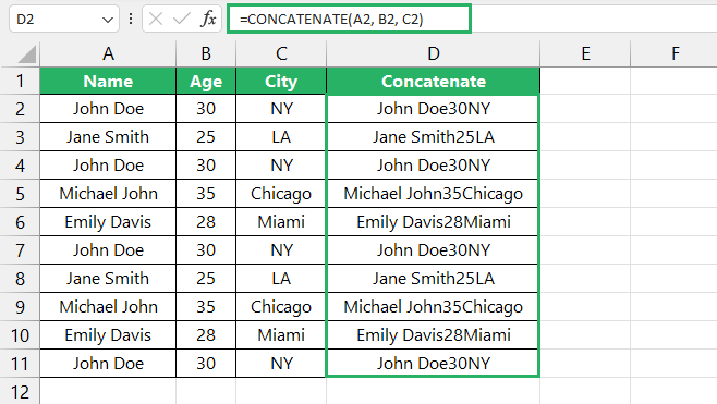
But we’re not done here. 🤓

Step 5) Select a new column – cell E2.

Step 6) Type in the COUNTIF function.

Step 7) Press Enter and copy the formula down using the Fill Handle.

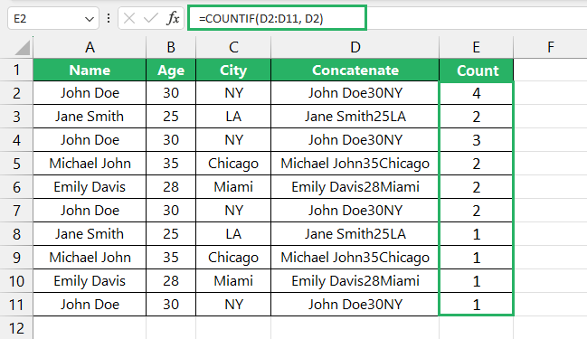
You will now be able to see the count of the duplicates in your data set.

To get rid of these duplicate values,

Step 8) Select the column header Count and right-click it.

Step 9) From the dropdown menu, select Filter.

Step 10) Select Filter by Selected Cell’s Value

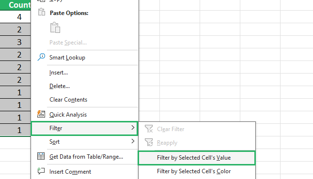
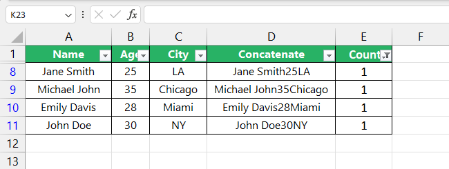
All the values in your data set will be hidden and your worksheet will look like this.

Step 11) Click on the Filter button in cell E1 and select 1 from the checkboxes.

Step 12) Press Ok 🆗

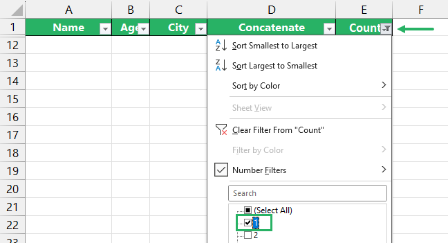
And it’s done. The Filter will now only display unique values in your data set and will omit all duplicate values.

Try it yourself now! 😃

Remove Duplicates in Excel Using the Remove Duplicates Feature

Apart from formulas, there are other ways you can remove duplicate values in Excel, and among them, the most popular is the Remove Duplicates Feature.

Unlike the formulas above, the Remove Duplicates feature deletes the duplicate rows within the range of cells you chose and doesn’t create a new column to store the unique values.

Let’s see a step-by-step on how to achieve that below.

Say, this is our sample data set.

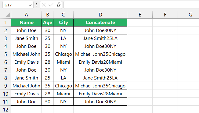
Step 1) Press Ctrl + A to select the entire range.

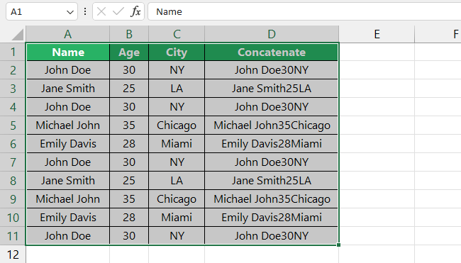
Step 2) Go to the Data tab on the ribbon.

Step 3) Click on the Remove Duplicates button under the Data tools section next to Text to Columns

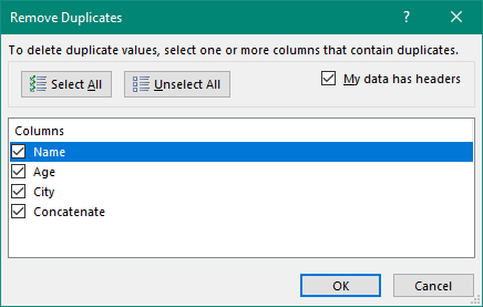
Step 4) The Remove Duplicates dialog box will appear on the screen.

Step 5) If you want to delete duplicate entries from all columns, press OK.

But if you want to delete partial rows only,

Step 6) Click on the Unselect All button.

Step 7) Now check the boxes you want to delete rows from.

Step 8) Press Ok.

Excel will show a prompt that tells how many duplicate values it found and removed and the unique ones.

Step 9) Press Ok.

And it’s done. Your worksheet will now look something like this with all the duplicate rows deleted.

Remove Duplicates in Excel Using the Advanced Filter Feature

Another way of removing duplicate cells in Excel is to use the Advanced Filter feature. It works similarly to the Remove Duplicate option.

The only difference is that Advanced Filter gives you the choice of copying your unique values to a new column entirely or keeping them in the same location. This can be helpful if you just want to keep the original data intact.

Let’s see how to use this below.

Say, we have the following sample data.

Step 1) Select your entire data set.

Step 2) Go to the Data tab.

Step 3) Click on Advanced under the Sort & Filter section.

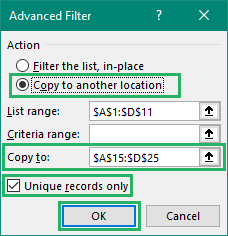
Step 4) A small Advanced Filter dialog box will appear on the screen.

Step 5) Under Action, select Copy to another location if you want your original data to remain unchanged.

Step 6) In the Copy to bar, select the column where you want the unique values to appear.

Step 7) Check the Unique Records only box at the bottom.

Step 8) Once done, press OK.

The data set with Unique values will appear on your worksheet as:

How cool is that? Try it now!

Conclusion

In this tutorial, we saw how to remove duplicates in Excel using different methods. We saw how to use formulas, built-in Excel features, and even the Advanced Filter option.

Removing duplicates is an important part of data cleaning in Excel and is a skill you mut have if you are an Excel user.

By following through, you should now be able to remove duplicates in all Excel spreadsheets regardless of the size. Read more about duplicates in Excel below

How to Find Duplicates in Excel

How to Use FILTER Function in Excel

How to Clear All Filters in Excel

We hope you enjoyed reading this article as much as we enjoyed creating it.