How to Filter Multiple Columns in Excel

When it comes to data management and analysis, Excel truly is incomparable. One of its most powerful features is its Filter which lets you focus only on the parts of information you want.

However, you understand the true power of Excel’s filter when you need to apply it across multiple columns with different criteria 🤔

Knowing how you can use filters to cater to different purposes can streamline your workflow and make you the go-to person for filtering data in Excel in your office.

In this tutorial, we will see various methods you can use to filter multiple columns simultaneously. Download our sample workbook here to practice along 🔽

Table of Contents

Filter columns using Sort & Filter

The most common way of filtering in Excel is to use the Sort & Filter feature. All you need to do is select your range and apply the filter. It’s that easy 😃

We will use the following sample dataset for this example. We want to see only the people working in HR and in those, we want to see the ones with a performance score above 90.

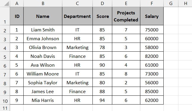
To do that,

Step 1) Select the range you want to apply filters to.

Step 2) Go to the Home tab, and select Sort & Filter from the Editing section.

Step 3) Select the filter from the dropdown menu that appears 📄

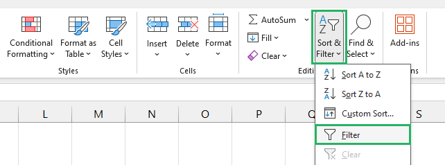
Step 4) The filter will appear on the selected range as a small funnel icon at the right bottom corner of the header.

Pro tip

You can do the same using the right-click menu too. Select the range you want to apply the filter to, right-click and select Filter. All the values in your dataset will be hidden for a while. The remaining process is the same.

Step 5) Click that funnel icon for HR.

Step 6) Click the Select All option under the search bar to unselect all options.

Step 7) Now select HR from the options.

Step 8) Press Ok.

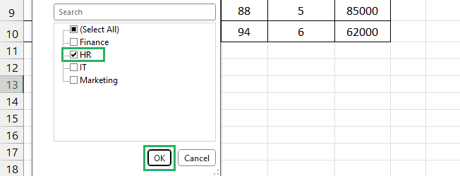
Step 9) All rows with HR in the Department column will show up.

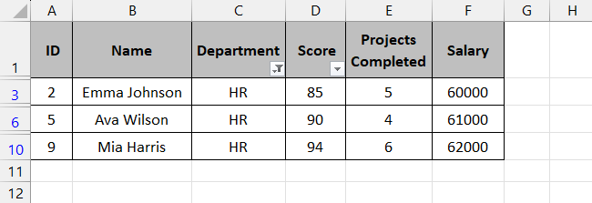
Step 10) Now, select the funnel on the Score column header.

Step 11) Select the checkboxes with values greater than 90.

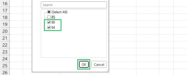
And it’s done! The auto filter will show only the rows that match the specified criteria.

How cool is that? 🤓

Filter columns using Advanced Filter

Another fun way you can use to filter multiple columns in one go is to use the Advanced Filter feature in Excel.

It lets you create complex criteria for filtering out your dataset in a rather simple way 😵

We will use the same sample dataset as earlier with the same objective. The criteria range is:

To do that,

Step 1) Click on any cell in your worksheet.

Step 2) Go to the Data tab and Select Advanced from the Sort & Filter section.

Step 3) The Advanced Filter dialogue box will appear on the screen.

Step 4) Under Action, select where you want the Filtered range to appear – we chose to filter in place.

Step 5) In the List range, select the range of your dataset to be filtered.

Step 6) In Criteria range. Select the range containing the criteria for filtering.

Step 7) There’s no need to check Unique Record Only.

Step 8) Press Ok 👍

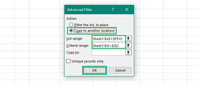
Voila! Both the targets have been achieved in one go.

The Advanced Filter shows rows with the department as IT and then filters them out further to only show the rows with a performance score equal to or above 85.

You can also change the criteria to display all the rows that have IT in them and have a performance score equal and above 85.

The criteria range for this example would be something like this:

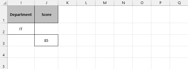
And the filtered dataset returned would be:

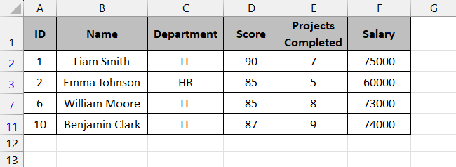
How simple is that? Try now! 😃

Filter columns using the FILTER function

You can also use the Excel FILTER function to filter multiple columns in one go. It takes a couple of arguments and returns the rows containing the given strings.

Its syntax is given as follows:

where,

array refers to the range to be filtered

include refers to a range comparable to an array

if-empty refers to the value to be returned if the array is empty or the filter returns nothing

We will use the same data set as earlier and will display the rows containing HR and a performance score greater than 90 🚩

To do that,

Step 1) Select cell H2.

Step 2) Enter the following formula in the cell:

Step 3) Press Enter.

The formula will display the rows with the above criteria as:

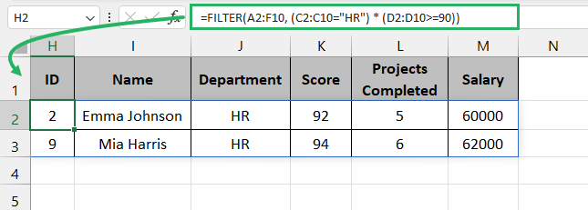
Wasn’t that easy? 🧐

Filter columns using Pivot Table

A pivot table is a creative way of filtering multiple columns in one go. It takes all your data and presents it in a composed form. You can select what data you want to show and what to filter.

We will use the same dataset as earlier. We want to display all the rows containing the department finance with a score under 90.

To do that,

Step 1) Select your entire dataset.

Step 2) Go to the Insert tab, and select Pivot Table from the Pivot Table section.

Step 3) The Pivot Table dialog box will appear.

Step 4) Select the location of your pivot table – we chose a new sheet 📗

Step 5) Ensure the selected range is correct.

Step 6) Press Ok.

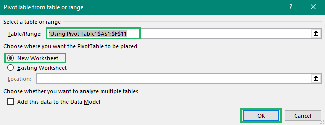
Step 7) Excel will take you to a new sheet with an empty pivot table.

Step 8) The pivot pane will appear on the right side of the sheet.

Step 9) Select the column names and drop them to the corresponding areas – this is the setting we used since department and score columns are to be filtered.

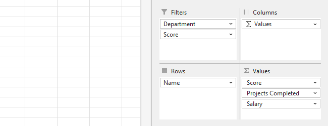
Step 10) The Department and Score label will appear at the top right corner of the sheet.

Step 11) Click the Department funnel and click on Select Multiple Items then select Finance 💰

Step 12) Click the Score funnel and select scores >90 by checking Select Multiple Items.

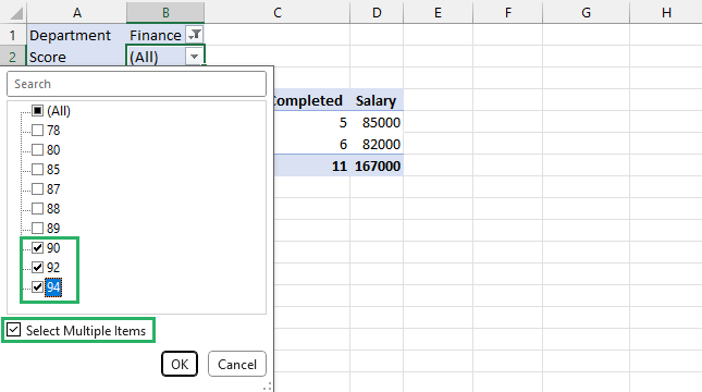
Step 13) You can now shift the Department column to the Names areas to display Finance in the pivot table.

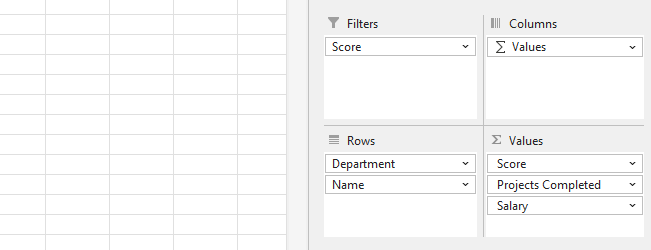
And it’s done! This is what the final pivot table looks like all filtered:

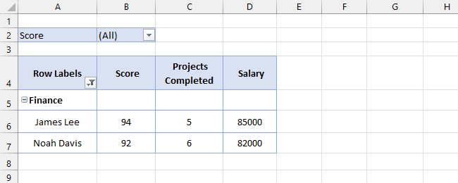
Pretty easy, right? You can do this for other columns too 😃

Pro tip

If you want a cleaner look of your pivot table, rename the columns in the Values area since they are often written with Sum of or Count of Prefix. Also, remove the Subtotals and Grand Totals from the pivot table if you don’t want them. You can remove them from the Design tab under the Layout section.

Filter columns using VBA

Another method you can use to filter multiple columns in one go is to use the VBA. It uses macros to perform a certain task.

VBA is an advanced level and is not recommended for beginners as it might be slightly difficult to understand 🤔

We have the same sample data as earlier. We want to display rows containing HR and scores above 90.

To do that,

Step 1) Press Alt + F11 on your keyboard

Step 2) The Visual Basic editor will appear on the screen.

Step 3) Go to the Insert tab and select Module.

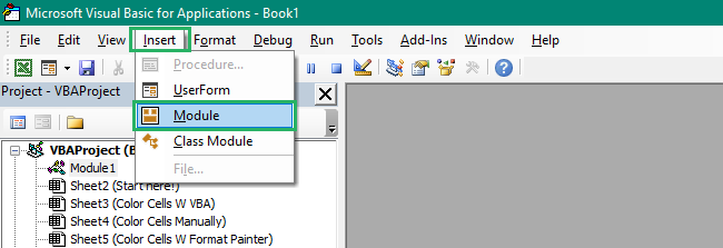
Step 4) Paste the following code into the window.

Step 5) Close the editor.

Step 6) Press Alt + F8 to open the Macros windows.

Step 7) Select FilterMultipleColumns and press Run 🏃‍♀️

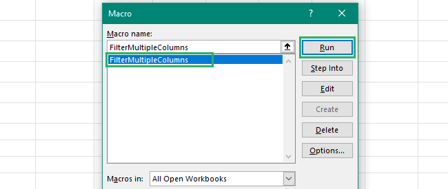
All rows will be hidden with only the ones being displayed meeting the criterion.

Smooth, no? 😉

Conclusion

In this guide, we saw different methods on how to filter multiple columns in Microsoft Excel. We saw how you can use filters using auto and advanced filters and conditional formatting 🎨

We also saw how you can achieve the same results using a pivot table, FILTER function or VBA. Filter is a vital Excel feature that is always used when dealing with datasets – whether large or small.

To learn more about filters, and pivot tables, read these articles below.

How to Use the FILTER Function in Excel + Examples (2024)

How to Clear All Filters in Excel in 1 Minute (2024)

How to Create a Pivot Table in Excel: Step-by-Step (2024)

We hope you enjoyed reading this piece as much as we did crafting it! 🤗