How to Use Data Validation in Excel: Full Tutorial
Sometimes we have to share our Microsoft Excel files with multiple users to fill in data.
The problem with sharing Excel files is that other people might input the wrong data. Which in turn screws up filtering, lookups, and other types of features and functions.
To prevent this, use data validation!
And I’ll walk you through how to do that here, step-by-step, in this table😊

If you want to tag along, download the practice workbook here.
Table of Contents
What is data validation in Excel?
Excel data validation helps to check input based on validation criteria. 🤔
That means data validation can be used:
- To check if a value is a number, a date, a time, a text with a specified length or
- To show a dropdown menu to the user with set options.
As a result, it can help users enter only valid data into a cell.🤗
You can also show a custom message to the user before entering data into a cell.
You can also display a warning message if the users enter invalid data.
This will simplify data entry and minimize input and typing errors. 😊
Before using Excel’s data validation feature on our table, we shall become familiar with it.👍
How to add data validation
- To start, you have to select one or more cells in the Excel file for data validation.
- Then, go to the data tab.

- Click the data validation button, in the Data Tools Group, to open the data validation settings window.
This is how the data validation window will appear.
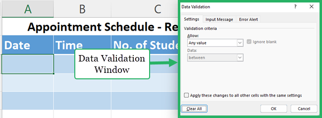
- The first tab in the data validation window is the settings tab.
You can create rules for data validation in this tab.
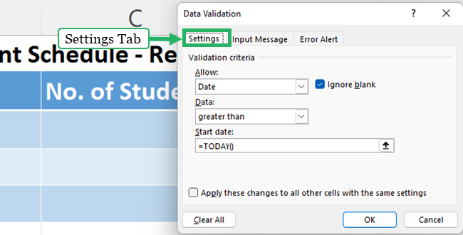
For example, we can specify that the date in the first column must be a future date.
In the following part, we will go through all of the data validation rules in depth🤗.
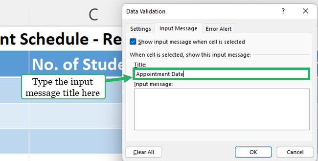
- Go to the input message tab to create an input message.
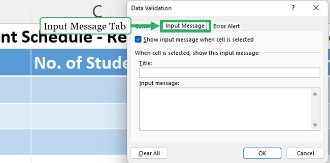
Put a tick mark for the “Show input message when cell is selected”.
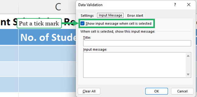
Input messages can be a guide to user input data in the correct format and reduce entering invalid data.
Add a title for the input message.
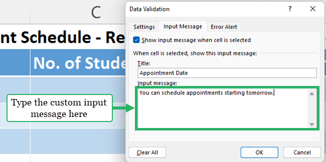
Enter a custom message for the input message.
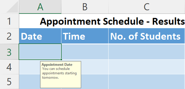
When you select a cell with data validation, you will see an input message similar to this.
- Finally, go to the error alert tab to create an error message for invalid data.
When a user enters an invalid entry or invalid value, you can show an error alert.
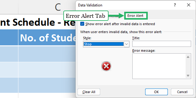
Put a tick mark next to the “show error alert after invalid data is entered” in the error alert tab.
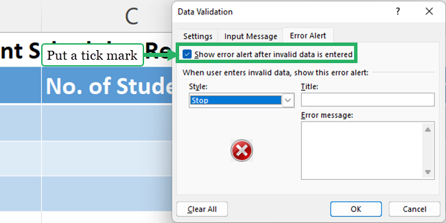
You can select 3 different styles for the error message when a user inputs invalid data.
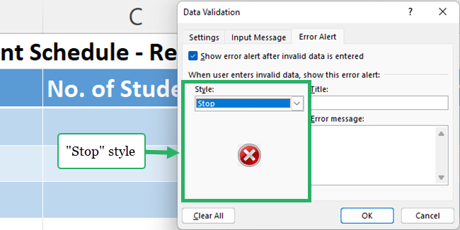
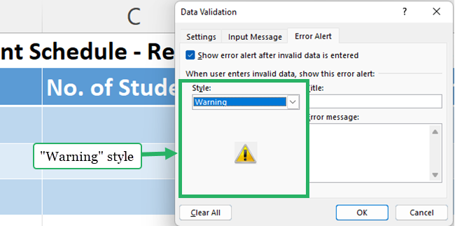
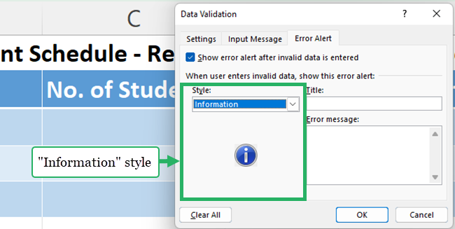
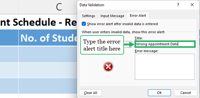
Next, give a title to your error alert.
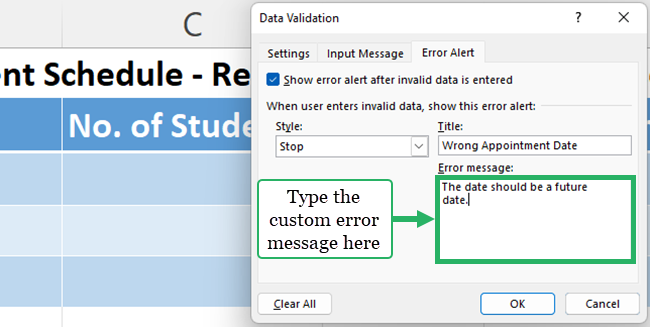
Then, enter a custom error message.
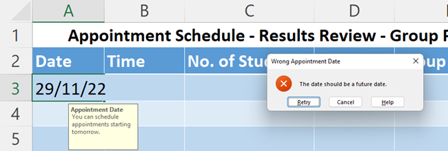
This error message will show up if a student enters a date that has passed.
Let’s apply data validation rules to our Excel data table.
Types of data validation rules
Dates and time validation rules
Date data validation rule
Students can make an appointment date only for a future date.
Let’s learn how to avoid entering an invalid date in the date column.
- Select “date” from the allow box in the settings tab.
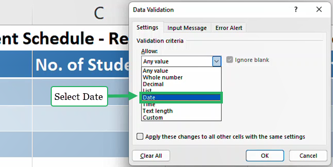
By selecting “date”, restrict data entry types to date in the validation cell.
- Select a condition under the data drop down list and specify data validation criteria in the start date box.
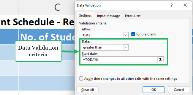
Students can now only enter future appointment dates in the first column of the Excel table.
Time data validation rule
Next, we want to make sure that students enter appointment times between 8 a.m. and 5 p.m.
- Select “Time” as the data validation criteria from the allow box.
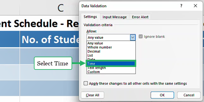
By selecting “Time”, all other entries other than time will become invalid entries in data validation cells.
- Select a condition under the data drop down list in the data validation dialog box.
Then enter the data validation rule for the time column.
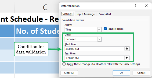
Pro Tip!
How to change data validation settings for many cells easily?
No need to copy data validation one by one.
You can check the below box to apply the changed data validation settings to all cells with the same settings.
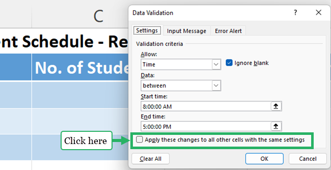
Number validation rules
Whole number data validation rule
We want to make sure that no more than three students attend the appointment.
In other words, we need to create an error message as invalid data if the data entry is not a whole number or is more than 3.
Let’s learn how to apply the whole number validation rule.
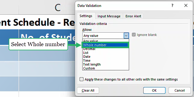
- Select the “Whole number” as the data validation criteria from the settings tab.
- Select a condition under data in the data validation dialog box.
I select “between” and give 1 & 3 as the minimum and maximum values.
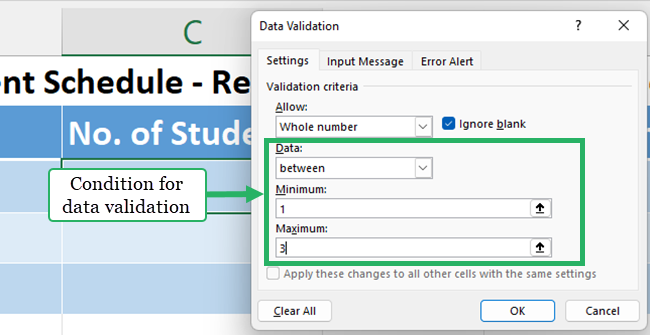
Students can enter only 1, 2, or 3 in column C.
Decimal data validation rule
We would like to get the group results when they are scheduling the appointment.
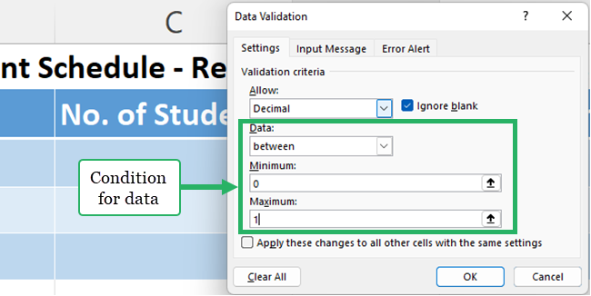
The results should be between 0% to 100% (i.e., the results should be between 0 to 1).
Let’s learn how to do data validation in excel for decimal values.
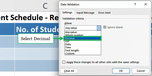
- Select “Decimal” as the data validation criteria from the settings tab.
- Select a condition from the list under data and apply validation criteria.
Text validation rule
Do you think we can have data validation in Excel only for numeric values?🤔
No. We can apply for data validation in excel for text length as well.
When the user inputs a text that has a different length to the given data validation that data entry can be recognized as invalid data.
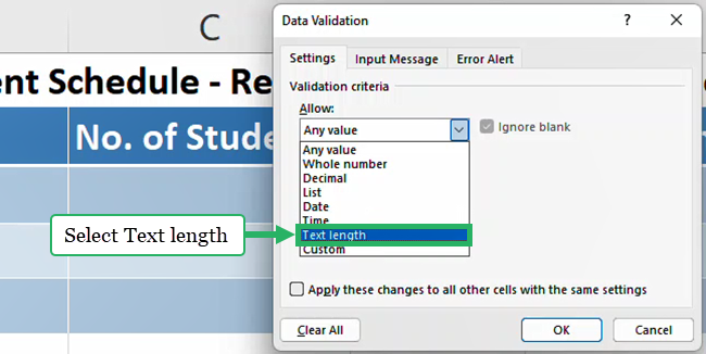
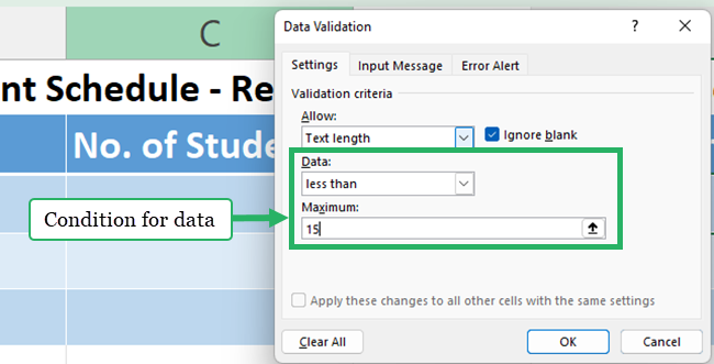
In this table, the group name should be less than 15 letters.
Let’s look at how we can validate the group name.
- Select the “Text length” as the data validation criteria from the settings tab.
- Select a condition for the data validation from the data box.
Drop-down lists
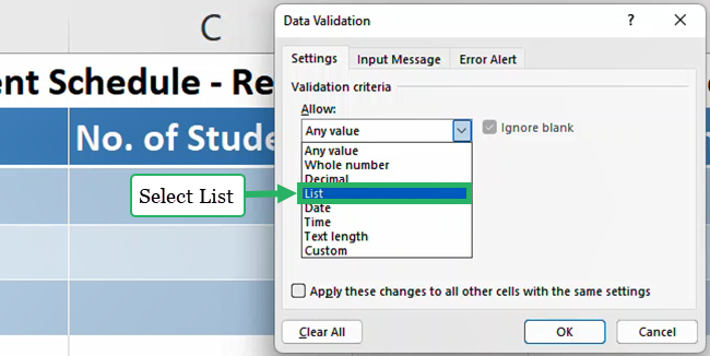
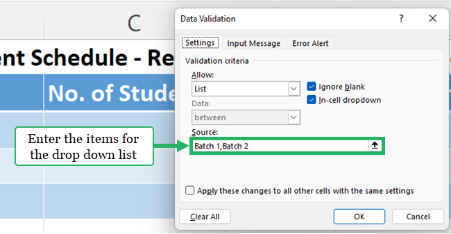
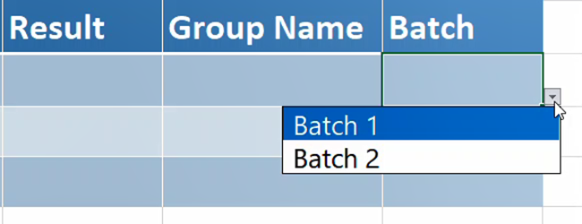
In the last column, students must enter either “Batch 1” or “Batch 2”.
We can give those 2 options in a cell dropdown box.
If the user selects “Batch 1”, it will show in that cell.
Let’s learn how to create a drop down list.
- Select the “List” as the data validation criteria.
- Enter the items for the drop down list in the source box or give a specified range for the drop down list in the source box.
To give a cell reference, click the upside arrow in the source box.
Pro Tip!
Is it difficult to update drop down list, if the number of options for drop down list are changing every time?😕
Don’t worry.
Give the cell reference of the source box to a Table in Excel.
The table automatically updates your list.😍
With the drop down list, users can easily select the batch.
Since drop down list is a very common data validation feature, it is good to learn this in a very detailed manner.
I highly recommend checking out my drop-down tutorial here to learn all about it!
Now users can enter only valid entries into our Excel table.
How to remove data validation
Now you know how to apply data validation in excel.👏
Do you want to know how to remove data validation?
It is very simple!🙂
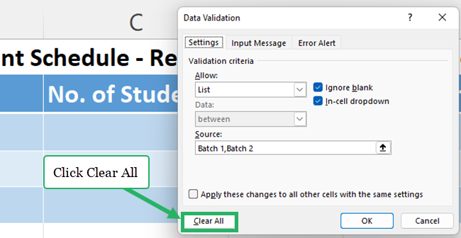
- Select the cells that contain data validation you need to remove.
- Go to the data tab
- Click on the data validation icon.
- Click “Clear All”.
That’s it – Now what?
Now, you can easily add data validation to your cells, making it almost impossible for other users to mess up data input 😊
Pretty great, right?
But messed up data is only a problem if there’s something relying on that data.
Functions like IF, SUMIF, and VLOOKUP rely on data being neat and orderly. And those functions are the backbone of most important spreadsheets.
If you don’t master them yet, click here to learn IF, SUMIF, and VLOOKUP in my free 30-minute online course.
Other resources
If you want to use more advanced date and time functions as validation conditions, read our article about Excel’s Date and Time Functions.
After applying data validation, it is quite simple to narrow down your data to find what is relevant with Excel Filters. Read our How to Filter in Excel article to find out more information about the Excel filter tool.
And not just that! When you have complete data, you can easily rearrange it using Pivot Tables.
