How to Write a Formula in Excel
(Beginner Tutorial)
Excel is all about running calculations! And so creating and operating a formula in Excel is simple.
An Excel formula is a combination of operators and operands. For example, 2 + 2 = 4 is a formula where 2s are the operands, plus sign (+) is the operator, and 4 is the answer to the formula.
Only if you know the basics to write a formula in Excel – there’s a high chance you’d solve most of your Excel problems. This article explains the basics of creating Excel formulas.
So let’s dive right in.
As you scroll down, download our free sample workbook here to practice the examples used in the guide below. 😀
Table of Contents
How to create formulas in Excel
Creating Excel formulas is easy as pie.
For example, what is 10 divided by 2? Can you calculate this in Excel?
1. Start by activating a cell.
2. Write an equal sign.
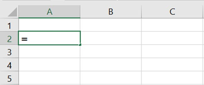
It is very important to start any formula with an equal sign. If you do not start with an equal sign, Excel wouldn’t recognize it as a formula but as a text string.
3. Input the simple mathematical operation of 10 divided by 2.
= 10 / 2
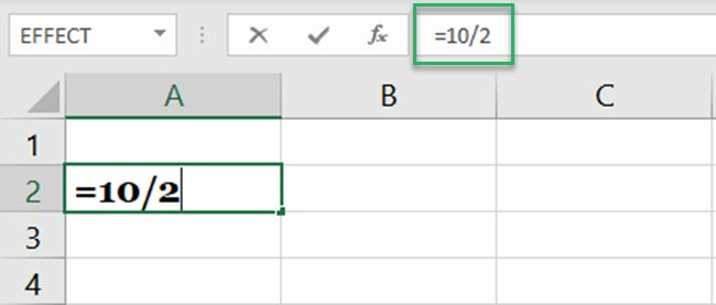
4. Hit enter, and you’re good to go!
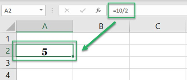
You can create the same above formula with a slight variation.
For example, if you have the operands as cell values.
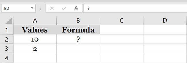
1. Write the formula using cell references as follows.
= A2 / B2
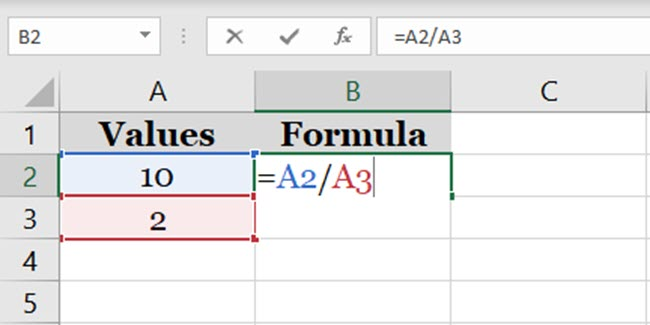
The above formula translates to ‘A2 divided by A3’.
Where A2 has the numeric value 10, and A3 has the numeric value 2.
2. The results remain the same as in the above example.
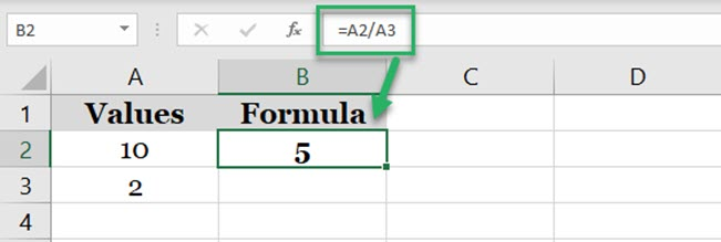
Creating a formula using cell references and values
The same formula can also be created using a combination of cell references and values.
Write the following formula using cell references and values.
= A2 / 2
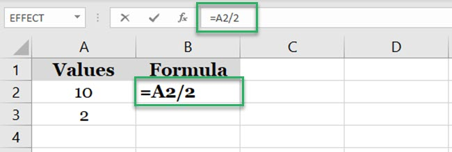
The above formula translates to ‘A2 divided by 2’.
Where A2 has the numeric value 10, and 2 is a value.
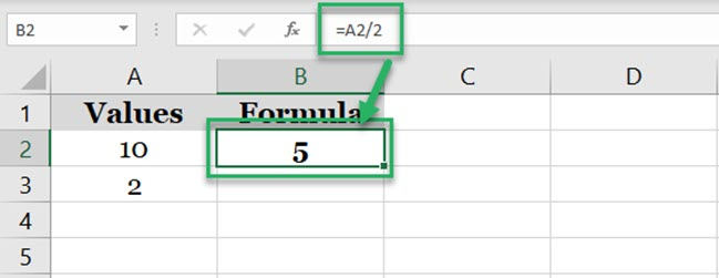
1. The results look as follows.
Pro Tip!
Using cell references is better than using absolute values. This is because if sometime later you change the cell value – the formula would automatically update.
How to add, subtract, multiply, and divide?
There are four basic mathematical operations – add, subtract, multiply, and divide.
Let’s now see how to perform each of these operations in Excel.
How to make a SUM formula (addition)
Adding things up in Excel can take different forms.
Excel has an in-built function for performing addition i.e. the SUM function. Here’s how you can bring it to action.
1. Write the SUM function beginning with an equal sign as follows.
= SUM (5, 5)
Every argument of the SUM function separated by a comma represents the value to be added.
Excel adds 5 into 5 to give the results below.
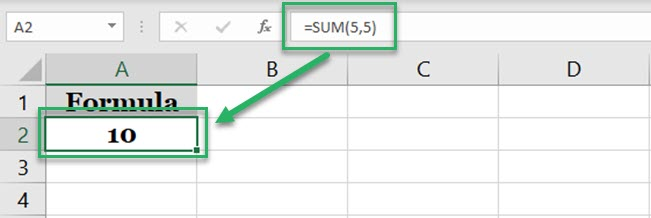
Easy enough? You can use the SUM function for cell references too. 🤩
2. Write the SUM function as follows.
= SUM (A2, A3)
Pro Tip!
To insert SUM from the Insert Function button, take this route.
Go to Formulas tab > Function Library > Insert function button > Type the function name.
In the Insert Function dialog box, type SUM and hit search. Select the desired function and hit ‘Okay’ to insert the same.
Excel adds the cell values of Cell A2 and Cell A3.
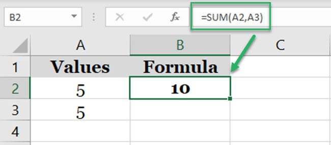
What makes the SUM function a big plus is its ability to add up a range of cells.
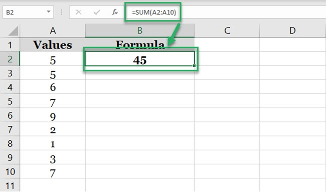
For example, see the data below.
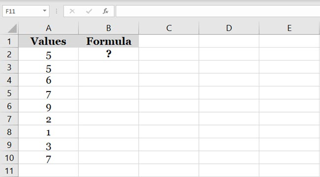
3. To add this up in Excel using the SUM function, write the SUM function as below.
= SUM (A2:A10)
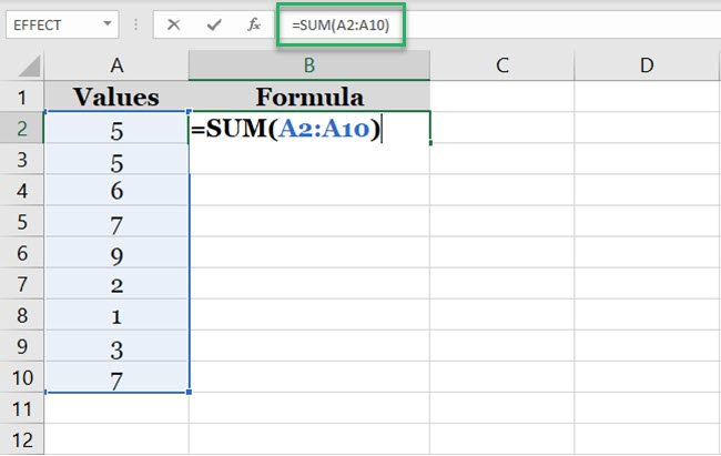
Must notice how we have defined the cell range from Cell A2 to Cell A10 as A2:A10.
4. Excel sums up all cell values in cells from A2 to A10.
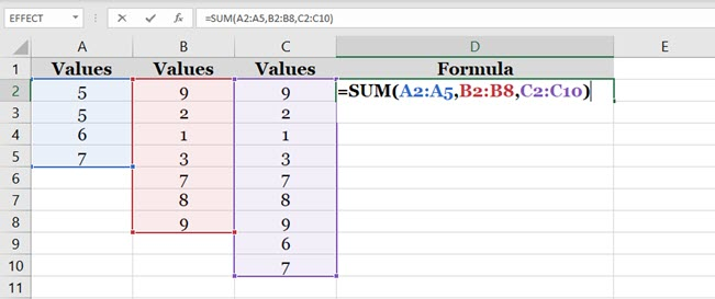
You can make this function work even more interestingly by adding up multiple ranges.
5. Write the SUM function with multiple ranges as follows.
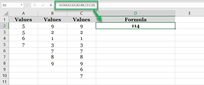
= SUM (A2:A5, B2:B8, C1:C10)
Here are the results.
How to subtract in Excel
Subtracting in Excel is all about creating a formula with the minus sign operator (-).
For example:
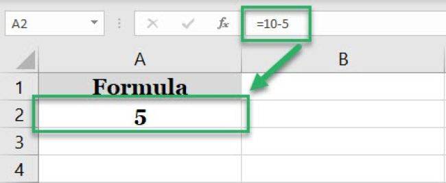
1. To subtract 5 from 10, begin with an equal sign and write the following formula.
= 10 – 5
A simple subtraction formula with a minus sign operator!
Press enter and here you go.
2. Try doing the same with cell references as below.
= A2 – A3
This formula translates to A2 less A3. Where A2 has the numeric value 10, and A3 has the numeric value 5.
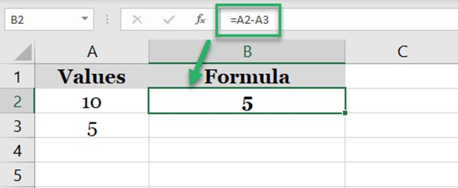
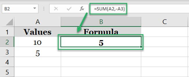
3. Alternatively, you can use the SUM function to perform subtraction. However, to do this you need to add a minus sign to the value to be subtracted.
= SUM (A2, -A3)
Here are the results.
How to multiply in Excel
After we have learned how to add and subtract in Excel, it’s time we learn multiplication in Excel.
First thing first, the operator for multiplication in Excel is an asterisk (*).
Now, do you remember what is 9 times 8? No?
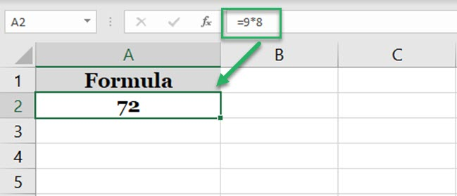
1. Write a multiplication formula in Excel.
= 9 * 8

Excel multiples 9 and 8.
2. Try doing the same using cell references as below.
= A2 * A3
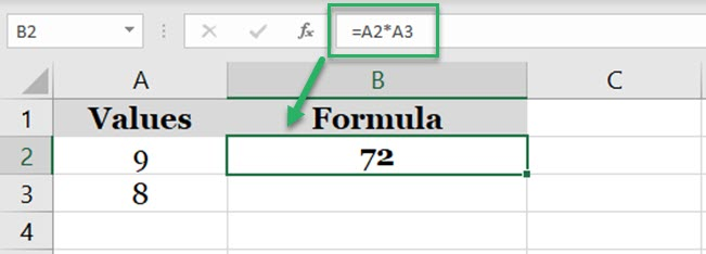
The formula above translates to A2 multiplied by A3.
Excel also offers an in-built function for multiplication in Excel. The PRODUCT Function!
3. Write the PRODUCT function as follows.
= PRODUCT (9, 8)
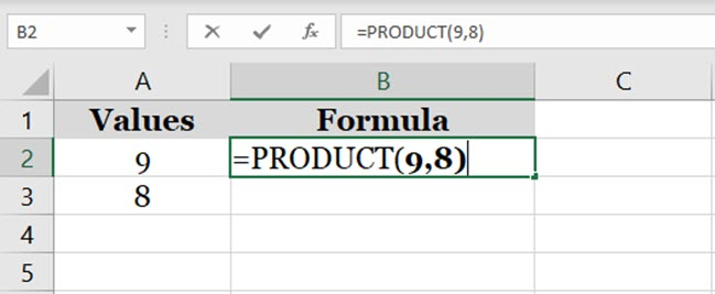
We have added both the values to be multiplied as the arguments to the PRODUCT function.
Here are the results.
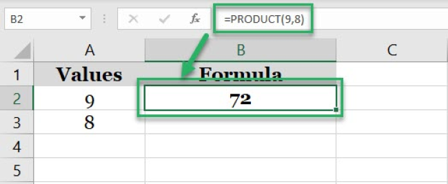
The PRODUCT function can also find the product of multiple values (or a range of cells) at once.
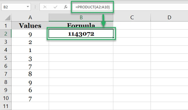
For example, see the data below.
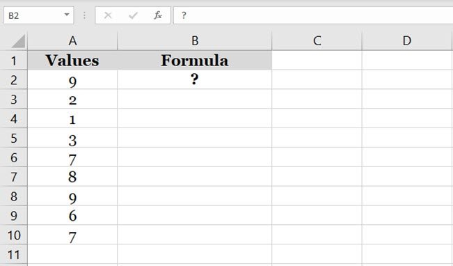
4. To multiply all these values, write the PRODUCT function as follows:
= PRODUCT (A2:A10)
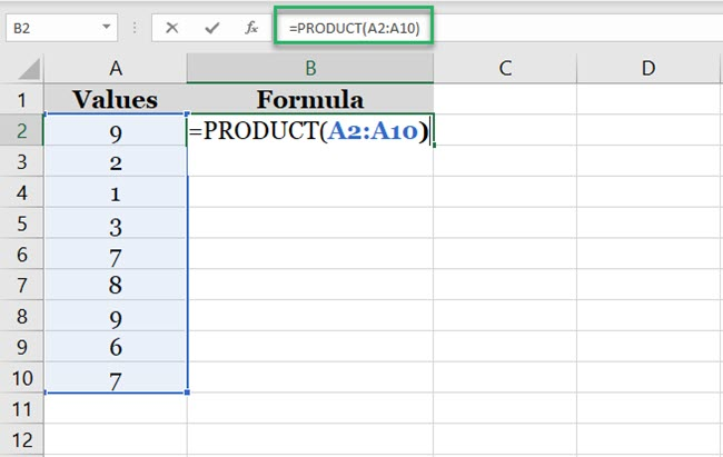
Excel multiplies all the values in the specified range.
How to divide in Excel
Here comes the last operation of this guide – division. 🤞
Creating a division formula in Excel is also very straightforward.
What is the operator for division? A forward slash (/).
Also, the dividend (or the numerator) comes before the slash. And the divisor (or the denominator) comes after the slash.
1. Write a division formula as below.
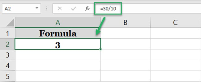
= 30 / 10
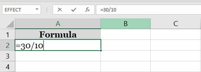
Excel divides both operands to give the results as follows.
2. The same can be done using cell references.
= A2 / A3

Pro Tip!
While performing the division function in Excel, you might see the #DIV/0! Error. This error is given back by Excel when you attempt to divide the number of zero.
Basic Rule of Grade 6! No number is divisible by zero. Excel remembers that, if not us. 😆
Order of operations
Here’s an equation for you to solve.
= 2+ 4 * 6 / 3 – 2
What a mess! Which operation do you perform first?
To solve this mystery, there is an order for performing mathematical operations – PEMDAS
P = Parenthesis
E = Exponents
MD = Multiplication & Division (left to right)
AS = Addition & Subtraction
Solve the above equation in the same order, and you’d reach the answer 8.
Let Excel do the same to see the results.
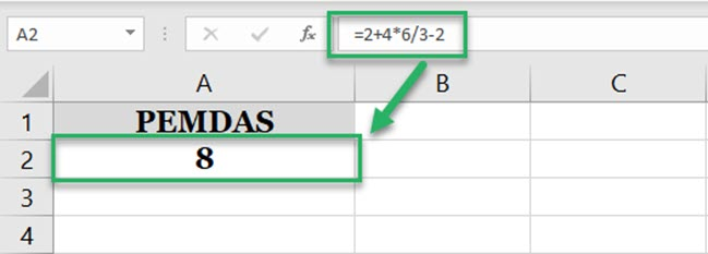
Excel performs division first (6 / 3 = 2), multiplication second (4 * 2 = 8), addition third (2 + 8 = 10), and subtraction last (10 – 2 = 8), resulting in 8.
Now, let’s enclose a part of this formula in parentheses to see how the results change.
= 2+ 4 * 6 / (3 – 2)
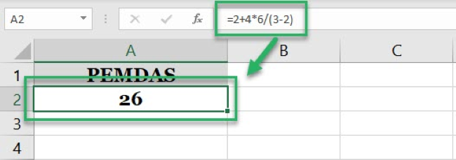
What causes the results to change with only parenthesis added?
Excel now first performs the operation enclosed in parentheses i.e. (3-2).
Next, multiplication is performed, then division and addition last. This causes the answer to change.
Pro Tip!
Try doing some mental maths to double-check if Excel has rightly calculated 26.
Parenthesis first = 2+ 4*6/(3 – 2)
Multiplication Second= 2+4*6/1
Division Third = 2 + 24/1
Addition Last = 2 + 24
Here’s the answer = 26
How to create formulas with references
Creating Excel formulas with references is super simple. All you need to do is replace the values in a simple formula with cell references (cells that contain those values).
For example, let’s create a multiplication formula in Excel.
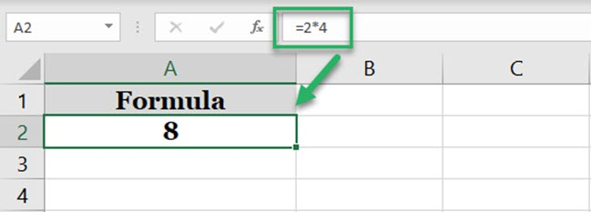
Great! What if you had 2 & 4 as numerical values in cells?
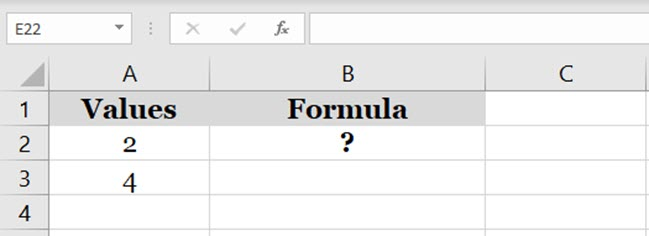
Create the same formula using cell references.
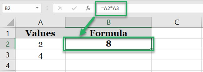
You can do the same for all operators! It is this simple.
Also, what happens when a cell value changes? Until the cell reference is in place, the formula would automatically update for the cell value change.
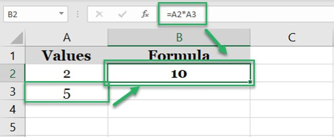
Must note how the cell reference in the formula remains unchanged. The answer however changes as the cell value for A3 has changed.ltiple criteria lookup💡
Formulas or functions?
What is an Excel formula, and what is an Excel function? And how are these two different?
There are two ways to add 2 and 2 in Excel.
- = 2 + 2
- SUM (2,2)
The answer to them both would be the same. However, the first one is a formula created in Excel. Whereas the second one is an in-built function of Excel – the SUM function.
Functions are more like predefined formulas in Excel.
Although the function library of Microsoft Excel is huge enough for you to explore, there is a limit to it. And you may not find everything you need there.
So, you might still need to write your own formulas to perform calculations in Excel. 😉
Pro Tip!
Sometimes, you might even nest a function into a formula.
For example, what is 2 + 2 – 3?
You may write it as = (SUM (2,2)) – 3
SUM (2,2) is a function, and deducting 3 from it makes it a self-created formula.
That’s it – Now what?
Until now, we’ve created formulas using different operators, values, and cell references. And learned how to use the SUM function for addition and subtraction.
Not only that but we’ve also studied the order of operations in Excel. The above article is a whole pack of information, isn’t it?
Creating your own formulas in Excel is the first step to manipulating numbers in Excel. However, this is something very basic, and Excel has tons more to offer.
Some very important Excel functions that one must hone include the VLOOKUP, SUMIF, and IF functions.
Haven’t mastered them yet? Click here to register for my 30-minute free email course that helps you learn these and much more.
Other resources
Found the above article interesting? Go ahead and check out other similar amazing articles of ours.
Read about Excel formulas being visible in cells, problems with Excel formulas not updating automatically, and errors posed by Excel.
