How to Highlight Duplicates in Excel (Step-by-Step)
There are several ways you can identify duplicates in Excel, you can do them by using Excel tools and even formulas.
However, one of the most persuasive ways to highlight duplicates is to highlight them (it’s catchy, and there’s no chance it will skip your sight 👀
The quickest way to identify and highlight duplicate values in Excel is the conditional formatting built-in option to highlight duplicate values. But, it is not the only one.
There are other methods too, and each of them has its unique relevance. To learn what these methods are and how can you leverage them to your good, download your free practice workbook for this guide here and continue reading till the end.
Highlight Duplicates in Excel with conditional formatting
Conditional formatting is a top-notch tool of Excel, and one of the best uses it brings to the table is highlighting duplicate values.
It is simple and quick. Let’s demonstrate this through the example below 👇
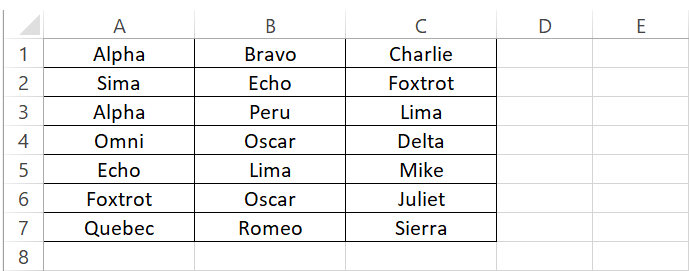
I have some data populated in a range of cells in Excel. Let’s quickly put together a conditional formatting rule to highlight duplicate values out of this set.
Step 1) Select the data.
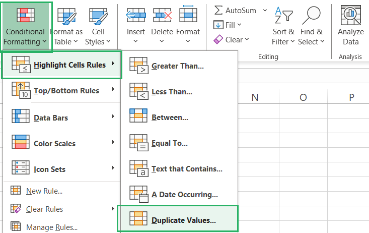
Step 2) Go to the Home tab > Styles group > Conditional Formatting.

Step 3) Click on it > Highlight Cells > Duplicate Values.
Step 4) From the Highlight Duplicate Values prompt, select the format with which you want the duplicate values highlighted from the predefined list of formats.
By default, it is set to red highlight with Dark Red text 🔴
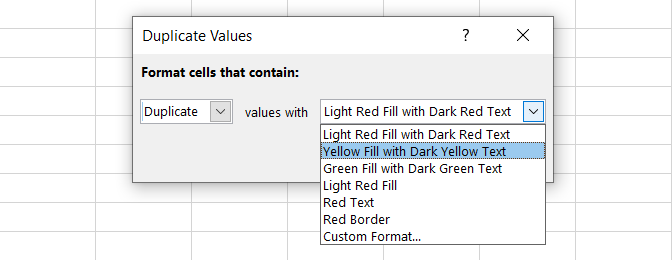
Step 5) Press okay and the duplicate values will be highlighted in the selected data.
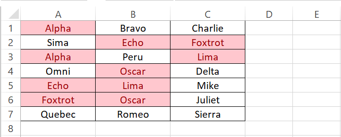
Conditional formatting is dynamic, and it automatically updates as the underlying data changes.
For example, if I copy and paste a value in this dataset, Excel will identify it as a duplicate and format it, too.
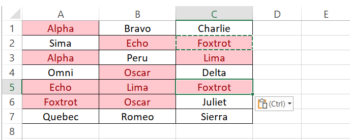
This makes conditional formatting easy and reliable.
Highlight Duplicates in Excel with the COUNTIF Function
We have seen how the conditional formatting to highlight duplicates in Excel works.
It highlights all those values that are present in the dataset more than once.
Another way to highlight duplicate values in Excel is to use the COUNTIF function. Under this method, you create a formula-based rule to identify and highlight duplicates 😲
Step 1) Select the data.
Step 2) Go to the Home tab > Styles group > Conditional Formatting > New Rule.
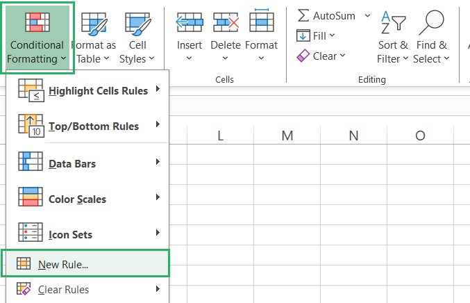
Step 3) In the New Formatting Rule box, select the option to “Use a formula to determine which cells to format”.
Step 4) In the space to enter a formula, write the following formula:
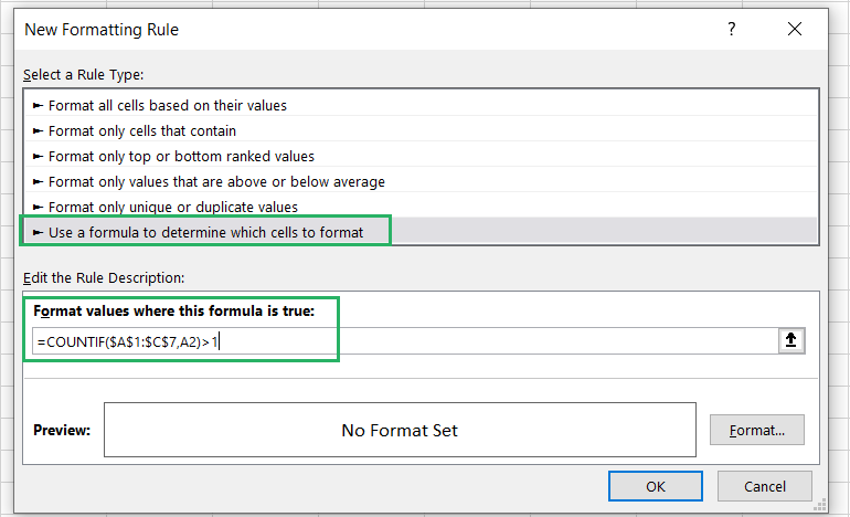
The COUNTIF function will check the whole range of cells containing the data against all the individual cells in the data and only count a cell where a cell value occurs more than once (instance of duplication).
Cells whose value appears more than once will then be highlighted 💡
To show you how this formula works, let me write it in simple cells:
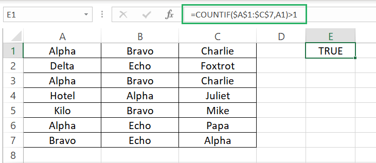
Now if I drag it down and sideways in the dimensions of our dataset, the cell range $A$1:$C$7 will not change as it is an absolute reference. But the criteria cell i.e., A2 will change for each successive cell.
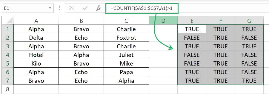
So COUNTIF checks if the cell ranges $A$1:$C$7 is equivalent to the cell value of the current cell (where the formula sits) for all the cells and returns TRUE for the cells whose value appears more than once in the data.
Step 5) Set the format for how you want the duplicate values to be formatted by clicking on the Format button.
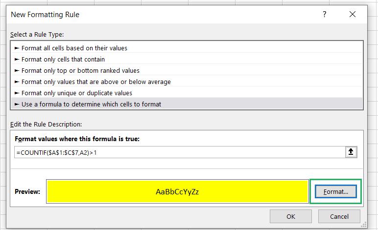
Step 6) Press okay to see Excel will highlight the duplicate entries.
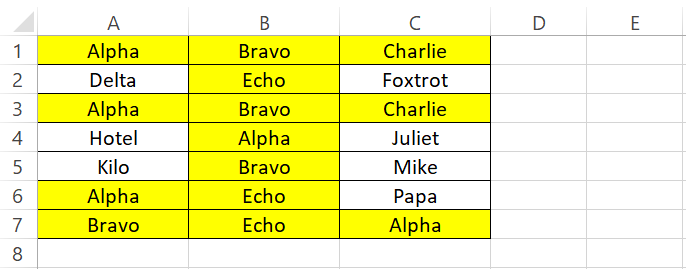
Until here, this method worked exactly as simple conditional formatting for highlighting duplicates does 🎯
However, this method outstands the rest as it allows highlighting not only duplicates but, also triplicates, quadruplicates, and so on.
See here.
In the data below, we have instances of duplication, triplication, and quadruplication 🤿
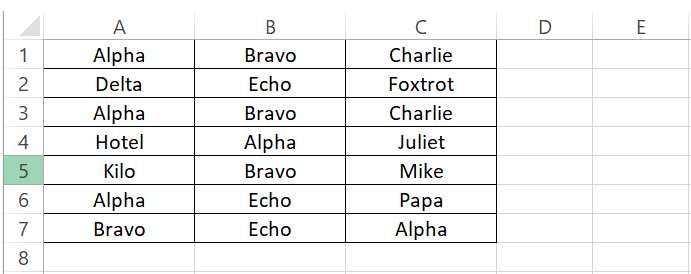
To highlight duplicates, we have already seen two methods above.
But if you want to highlight one triplicate (values that occur thrice or more), follow these steps:
Step 1) Select the data.
Step 2) Go to the Home tab > Styles group > Conditional Formatting > New Rule.
Step 3) In the New Formatting Rule dialog box, select the option to “Use a formula to determine which cells to format”.
Step 4) In the space to enter a formula, write the below formula:
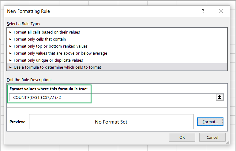
The COUNTIF function will not return true if the value in any cell occurs more than twice (triplicates) ⏭
Step 5) Set the format for how you want the triplicate values highlighted
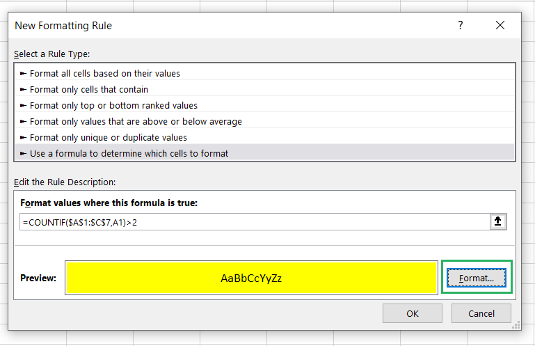
Step 6) Click the Okay button.
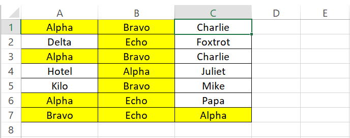
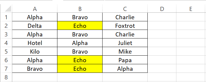
Note that “Charlie” was repeated twice in Cell C1 and C3 but, it was not highlighted. Only Alpha, Bravo, and Echo that occur thrice and (more than that) are highlighted.
Step 7) Similarly, define a rule with the COUNTIF function set to look for values that occur more than thrice.

Step 8) Click okay to see the values Excel highlights.
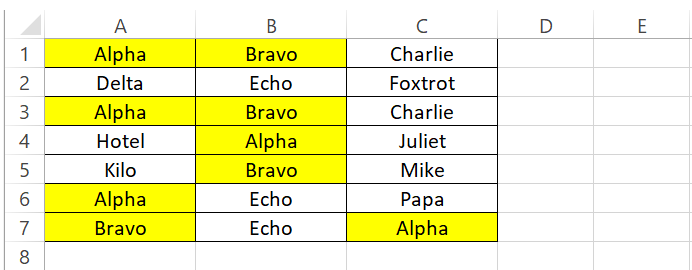
This is how the COUNTIF function leaves the highlighting reins in your hands.
Tweak the formulas in whatever way you want to define your own highlighting rule 🚴♀️
For example, if you only want Excel to highlight the cell values that appear thrice. Not more than that and not even any less than that:
Step 1) Open the New Rule Formatting window.
Step 2) Select the option to format cells based on a formula.
Step 3) Write the COUNTIF function as follows:
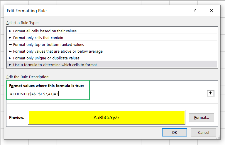
Excel will only highlight those values from the dataset that appear exactly thrice.
While you create new rules, select the underlying data and check the number of rules that apply to it by going to the Home tab > Styles group > Conditional Formatting > Manage Rules. Delete any other rules (that you applied previously but no longer need).
Conclusion
This tutorial covers some top-tier methods to find and highlight duplicates in Microsoft Excel. And not only duplicates, but triplicates, quadruplicates, and the versatile COUNTIF method that allows you to define the conditional formatting rules as you like them 🤍
We hope you enjoyed reading this tutorial and if you did, many other relevant Excel tutorials are waiting for you too. Hop on to the following links to check them out here.
